Repository of Reproducible Computations

Free Statistics

of Irreproducible Research!

Author's title

Author

*Unverified author*

R Software Module

rwasp_autocorrelation.wasp

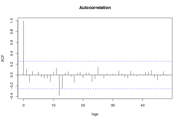
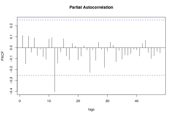
Title produced by software

(Partial) Autocorrelation Function

Date of computation

Sun, 21 Dec 2008 15:15:42 -0700

Cite this page as follows

Statistical Computations at FreeStatistics.org, Office for Research Development and Education, URL https://freestatistics.org/blog/index.php?v=date/2008/Dec/21/t1229897780bsrhxp4xib65mrd.htm/, Retrieved Sun, 18 Oct 2026 23:34:15 +0000

Statistical Computations at FreeStatistics.org, Office for Research Development and Education, URL https://freestatistics.org/blog/index.php?pk=35874, Retrieved Sun, 18 Oct 2026 23:34:15 +0000

QR Codes:

Paste this QR Code to cite your computation.

Original text written by user:

IsPrivate?

No (this computation is public)

User-defined keywords

Estimated Impact

561

Family? (F = Feedback message, R = changed R code, M = changed R Module, P = changed Parameters, D = changed Data)

F     [Variance Reduction Matrix] [Q2 VRM] [2008-12-07 13:38:56] [74be16979710d4c4e7c6647856088456]
F RMP   [(Partial) Autocorrelation Function] [Q2 ACF 00] [2008-12-07 13:48:21] [74be16979710d4c4e7c6647856088456]
F   P     [(Partial) Autocorrelation Function] [Q2 ACF 10] [2008-12-07 14:03:41] [74be16979710d4c4e7c6647856088456]
F   P       [(Partial) Autocorrelation Function] [Q2 ACF 11] [2008-12-07 14:10:14] [74be16979710d4c4e7c6647856088456]
- R PD        [(Partial) Autocorrelation Function] [] [2008-12-21 21:47:34] [74be16979710d4c4e7c6647856088456]
F   P             [(Partial) Autocorrelation Function] [] [2008-12-21 22:15:42] [d41d8cd98f00b204e9800998ecf8427e] [Current]
F RMP               [ARIMA Backward Selection] [] [2008-12-22 22:26:11] [74be16979710d4c4e7c6647856088456] 

Feedback Forum

2009-01-08 13:09:44 [Aurélie Van Impe] [reply] 
Je hebt goed opgemerkt dat er een sma proces van de eerste orde aanwezig is. Bij mijn weten is dit vrij duidelijk, ik zie niet in waarom je twijfelt.

Post a new message

Dataseries X:

Download CSV

Histogram

Boxplots

1.8
1.7
1.4
1.2
1
1.7
2.4
2
2.1
2
1.8
2.7
2.3
1.9
2
2.3
2.8
2.4
2.3
2.7
2.7
2.9
3
2.2
2.3
2.8
2.8
2.8
2.2
2.6
2.8
2.5
2.4
2.3
1.9
1.7
2
2.1
1.7
1.8
1.8
1.8
1.3
1.3
1.3
1.2
1.4
2.2
2.9
3.1
3.5
3.6
4.4
4.1
5.1
5.8
5.9
5.4
5.5
4.8
3.2

Summary of computational transaction
Raw Input	view raw input (R code)
Raw Output	view raw output of R engine
Computing time	1 seconds
R Server	'George Udny Yule' @ 72.249.76.132

\begin{tabular}{lllllllll}
\hline
Summary of computational transaction \tabularnewline
Raw Input & view raw input (R code)  \tabularnewline
Raw Output & view raw output of R engine  \tabularnewline
Computing time & 1 seconds \tabularnewline
R Server & 'George Udny Yule' @ 72.249.76.132 \tabularnewline
\hline
\end{tabular}
%Source: https://freestatistics.org/blog/index.php?pk=35874&T=0

[TABLE]
[ROW][C]Summary of computational transaction[/C][/ROW]
[ROW][C]Raw Input[/C][C]view raw input (R code) [/C][/ROW]
[ROW][C]Raw Output[/C][C]view raw output of R engine [/C][/ROW]
[ROW][C]Computing time[/C][C]1 seconds[/C][/ROW]
[ROW][C]R Server[/C][C]'George Udny Yule' @ 72.249.76.132[/C][/ROW]
[/TABLE]
Source: https://freestatistics.org/blog/index.php?pk=35874&T=0

Globally Unique Identifier (entire table): ba.freestatistics.org/blog/index.php?pk=35874&T=0

As an alternative you can also use a QR Code:

The GUIDs for individual cells are displayed in the table below:

Summary of computational transaction
Raw Input	view raw input (R code)
Raw Output	view raw output of R engine
Computing time	1 seconds
R Server	'George Udny Yule' @ 72.249.76.132

Autocorrelation Function
Time lag k	ACF(k)	T-STAT	P-value
1	0.111593	0.8644	0.195408
2	-0.13546	-1.0493	0.149132
3	0.067299	0.5213	0.302041
4	0.002621	0.0203	0.491935
5	0.055072	0.4266	0.335605
6	-0.03383	-0.262	0.397092
7	-0.054247	-0.4202	0.337923
8	-0.05934	-0.4596	0.323717
9	-0.122981	-0.9526	0.172306
10	0.061149	0.4737	0.318732
11	0.126243	0.9779	0.166032
12	-0.383488	-2.9705	0.002136
13	-0.253384	-1.9627	0.027161
14	0.031769	0.2461	0.40323
15	0.062439	0.4836	0.315198
16	-0.026597	-0.206	0.418738
17	-0.143171	-1.109	0.135927
18	0.04029	0.3121	0.378028
19	0.059906	0.464	0.322152
20	-0.055777	-0.432	0.333629
21	0.041166	0.3189	0.375466
22	0.039841	0.3086	0.379345
23	-0.124926	-0.9677	0.168547
24	-0.075186	-0.5824	0.281244
25	0.151689	1.175	0.122322
26	0.013049	0.1011	0.459913
27	-0.057953	-0.4489	0.327561
28	0.023823	0.1845	0.427108
29	0.010308	0.0798	0.468314
30	0.018272	0.1415	0.44396
31	0.001138	0.0088	0.496497
32	0.078392	0.6072	0.272996
33	0.026169	0.2027	0.420025
34	-0.035841	-0.2776	0.391129
35	-0.057637	-0.4465	0.328437
36	0.077023	0.5966	0.276504
37	0.026441	0.2048	0.419205
38	-0.019392	-0.1502	0.440551
39	0.013209	0.1023	0.459423
40	-0.002243	-0.0174	0.493097
41	0.047114	0.3649	0.358219
42	0.060538	0.4689	0.32041
43	0.088559	0.686	0.247687
44	-0.043536	-0.3372	0.368561
45	-0.094733	-0.7338	0.232965
46	-0.014624	-0.1133	0.455095
47	0.066145	0.5124	0.305142
48	-0.014	-0.1084	0.457002

\begin{tabular}{lllllllll}
\hline
Autocorrelation Function \tabularnewline
Time lag k & ACF(k) & T-STAT & P-value \tabularnewline
1 & 0.111593 & 0.8644 & 0.195408 \tabularnewline
2 & -0.13546 & -1.0493 & 0.149132 \tabularnewline
3 & 0.067299 & 0.5213 & 0.302041 \tabularnewline
4 & 0.002621 & 0.0203 & 0.491935 \tabularnewline
5 & 0.055072 & 0.4266 & 0.335605 \tabularnewline
6 & -0.03383 & -0.262 & 0.397092 \tabularnewline
7 & -0.054247 & -0.4202 & 0.337923 \tabularnewline
8 & -0.05934 & -0.4596 & 0.323717 \tabularnewline
9 & -0.122981 & -0.9526 & 0.172306 \tabularnewline
10 & 0.061149 & 0.4737 & 0.318732 \tabularnewline
11 & 0.126243 & 0.9779 & 0.166032 \tabularnewline
12 & -0.383488 & -2.9705 & 0.002136 \tabularnewline
13 & -0.253384 & -1.9627 & 0.027161 \tabularnewline
14 & 0.031769 & 0.2461 & 0.40323 \tabularnewline
15 & 0.062439 & 0.4836 & 0.315198 \tabularnewline
16 & -0.026597 & -0.206 & 0.418738 \tabularnewline
17 & -0.143171 & -1.109 & 0.135927 \tabularnewline
18 & 0.04029 & 0.3121 & 0.378028 \tabularnewline
19 & 0.059906 & 0.464 & 0.322152 \tabularnewline
20 & -0.055777 & -0.432 & 0.333629 \tabularnewline
21 & 0.041166 & 0.3189 & 0.375466 \tabularnewline
22 & 0.039841 & 0.3086 & 0.379345 \tabularnewline
23 & -0.124926 & -0.9677 & 0.168547 \tabularnewline
24 & -0.075186 & -0.5824 & 0.281244 \tabularnewline
25 & 0.151689 & 1.175 & 0.122322 \tabularnewline
26 & 0.013049 & 0.1011 & 0.459913 \tabularnewline
27 & -0.057953 & -0.4489 & 0.327561 \tabularnewline
28 & 0.023823 & 0.1845 & 0.427108 \tabularnewline
29 & 0.010308 & 0.0798 & 0.468314 \tabularnewline
30 & 0.018272 & 0.1415 & 0.44396 \tabularnewline
31 & 0.001138 & 0.0088 & 0.496497 \tabularnewline
32 & 0.078392 & 0.6072 & 0.272996 \tabularnewline
33 & 0.026169 & 0.2027 & 0.420025 \tabularnewline
34 & -0.035841 & -0.2776 & 0.391129 \tabularnewline
35 & -0.057637 & -0.4465 & 0.328437 \tabularnewline
36 & 0.077023 & 0.5966 & 0.276504 \tabularnewline
37 & 0.026441 & 0.2048 & 0.419205 \tabularnewline
38 & -0.019392 & -0.1502 & 0.440551 \tabularnewline
39 & 0.013209 & 0.1023 & 0.459423 \tabularnewline
40 & -0.002243 & -0.0174 & 0.493097 \tabularnewline
41 & 0.047114 & 0.3649 & 0.358219 \tabularnewline
42 & 0.060538 & 0.4689 & 0.32041 \tabularnewline
43 & 0.088559 & 0.686 & 0.247687 \tabularnewline
44 & -0.043536 & -0.3372 & 0.368561 \tabularnewline
45 & -0.094733 & -0.7338 & 0.232965 \tabularnewline
46 & -0.014624 & -0.1133 & 0.455095 \tabularnewline
47 & 0.066145 & 0.5124 & 0.305142 \tabularnewline
48 & -0.014 & -0.1084 & 0.457002 \tabularnewline
\hline
\end{tabular}
%Source: https://freestatistics.org/blog/index.php?pk=35874&T=1

[TABLE]
[ROW][C]Autocorrelation Function[/C][/ROW]
[ROW][C]Time lag k[/C][C]ACF(k)[/C][C]T-STAT[/C][C]P-value[/C][/ROW]
[ROW][C]1[/C][C]0.111593[/C][C]0.8644[/C][C]0.195408[/C][/ROW]
[ROW][C]2[/C][C]-0.13546[/C][C]-1.0493[/C][C]0.149132[/C][/ROW]
[ROW][C]3[/C][C]0.067299[/C][C]0.5213[/C][C]0.302041[/C][/ROW]
[ROW][C]4[/C][C]0.002621[/C][C]0.0203[/C][C]0.491935[/C][/ROW]
[ROW][C]5[/C][C]0.055072[/C][C]0.4266[/C][C]0.335605[/C][/ROW]
[ROW][C]6[/C][C]-0.03383[/C][C]-0.262[/C][C]0.397092[/C][/ROW]
[ROW][C]7[/C][C]-0.054247[/C][C]-0.4202[/C][C]0.337923[/C][/ROW]
[ROW][C]8[/C][C]-0.05934[/C][C]-0.4596[/C][C]0.323717[/C][/ROW]
[ROW][C]9[/C][C]-0.122981[/C][C]-0.9526[/C][C]0.172306[/C][/ROW]
[ROW][C]10[/C][C]0.061149[/C][C]0.4737[/C][C]0.318732[/C][/ROW]
[ROW][C]11[/C][C]0.126243[/C][C]0.9779[/C][C]0.166032[/C][/ROW]
[ROW][C]12[/C][C]-0.383488[/C][C]-2.9705[/C][C]0.002136[/C][/ROW]
[ROW][C]13[/C][C]-0.253384[/C][C]-1.9627[/C][C]0.027161[/C][/ROW]
[ROW][C]14[/C][C]0.031769[/C][C]0.2461[/C][C]0.40323[/C][/ROW]
[ROW][C]15[/C][C]0.062439[/C][C]0.4836[/C][C]0.315198[/C][/ROW]
[ROW][C]16[/C][C]-0.026597[/C][C]-0.206[/C][C]0.418738[/C][/ROW]
[ROW][C]17[/C][C]-0.143171[/C][C]-1.109[/C][C]0.135927[/C][/ROW]
[ROW][C]18[/C][C]0.04029[/C][C]0.3121[/C][C]0.378028[/C][/ROW]
[ROW][C]19[/C][C]0.059906[/C][C]0.464[/C][C]0.322152[/C][/ROW]
[ROW][C]20[/C][C]-0.055777[/C][C]-0.432[/C][C]0.333629[/C][/ROW]
[ROW][C]21[/C][C]0.041166[/C][C]0.3189[/C][C]0.375466[/C][/ROW]
[ROW][C]22[/C][C]0.039841[/C][C]0.3086[/C][C]0.379345[/C][/ROW]
[ROW][C]23[/C][C]-0.124926[/C][C]-0.9677[/C][C]0.168547[/C][/ROW]
[ROW][C]24[/C][C]-0.075186[/C][C]-0.5824[/C][C]0.281244[/C][/ROW]
[ROW][C]25[/C][C]0.151689[/C][C]1.175[/C][C]0.122322[/C][/ROW]
[ROW][C]26[/C][C]0.013049[/C][C]0.1011[/C][C]0.459913[/C][/ROW]
[ROW][C]27[/C][C]-0.057953[/C][C]-0.4489[/C][C]0.327561[/C][/ROW]
[ROW][C]28[/C][C]0.023823[/C][C]0.1845[/C][C]0.427108[/C][/ROW]
[ROW][C]29[/C][C]0.010308[/C][C]0.0798[/C][C]0.468314[/C][/ROW]
[ROW][C]30[/C][C]0.018272[/C][C]0.1415[/C][C]0.44396[/C][/ROW]
[ROW][C]31[/C][C]0.001138[/C][C]0.0088[/C][C]0.496497[/C][/ROW]
[ROW][C]32[/C][C]0.078392[/C][C]0.6072[/C][C]0.272996[/C][/ROW]
[ROW][C]33[/C][C]0.026169[/C][C]0.2027[/C][C]0.420025[/C][/ROW]
[ROW][C]34[/C][C]-0.035841[/C][C]-0.2776[/C][C]0.391129[/C][/ROW]
[ROW][C]35[/C][C]-0.057637[/C][C]-0.4465[/C][C]0.328437[/C][/ROW]
[ROW][C]36[/C][C]0.077023[/C][C]0.5966[/C][C]0.276504[/C][/ROW]
[ROW][C]37[/C][C]0.026441[/C][C]0.2048[/C][C]0.419205[/C][/ROW]
[ROW][C]38[/C][C]-0.019392[/C][C]-0.1502[/C][C]0.440551[/C][/ROW]
[ROW][C]39[/C][C]0.013209[/C][C]0.1023[/C][C]0.459423[/C][/ROW]
[ROW][C]40[/C][C]-0.002243[/C][C]-0.0174[/C][C]0.493097[/C][/ROW]
[ROW][C]41[/C][C]0.047114[/C][C]0.3649[/C][C]0.358219[/C][/ROW]
[ROW][C]42[/C][C]0.060538[/C][C]0.4689[/C][C]0.32041[/C][/ROW]
[ROW][C]43[/C][C]0.088559[/C][C]0.686[/C][C]0.247687[/C][/ROW]
[ROW][C]44[/C][C]-0.043536[/C][C]-0.3372[/C][C]0.368561[/C][/ROW]
[ROW][C]45[/C][C]-0.094733[/C][C]-0.7338[/C][C]0.232965[/C][/ROW]
[ROW][C]46[/C][C]-0.014624[/C][C]-0.1133[/C][C]0.455095[/C][/ROW]
[ROW][C]47[/C][C]0.066145[/C][C]0.5124[/C][C]0.305142[/C][/ROW]
[ROW][C]48[/C][C]-0.014[/C][C]-0.1084[/C][C]0.457002[/C][/ROW]
[/TABLE]
Source: https://freestatistics.org/blog/index.php?pk=35874&T=1

Globally Unique Identifier (entire table): ba.freestatistics.org/blog/index.php?pk=35874&T=1

As an alternative you can also use a QR Code:

The GUIDs for individual cells are displayed in the table below:

Autocorrelation Function
Time lag k	ACF(k)	T-STAT	P-value
1	0.111593	0.8644	0.195408
2	-0.13546	-1.0493	0.149132
3	0.067299	0.5213	0.302041
4	0.002621	0.0203	0.491935
5	0.055072	0.4266	0.335605
6	-0.03383	-0.262	0.397092
7	-0.054247	-0.4202	0.337923
8	-0.05934	-0.4596	0.323717
9	-0.122981	-0.9526	0.172306
10	0.061149	0.4737	0.318732
11	0.126243	0.9779	0.166032
12	-0.383488	-2.9705	0.002136
13	-0.253384	-1.9627	0.027161
14	0.031769	0.2461	0.40323
15	0.062439	0.4836	0.315198
16	-0.026597	-0.206	0.418738
17	-0.143171	-1.109	0.135927
18	0.04029	0.3121	0.378028
19	0.059906	0.464	0.322152
20	-0.055777	-0.432	0.333629
21	0.041166	0.3189	0.375466
22	0.039841	0.3086	0.379345
23	-0.124926	-0.9677	0.168547
24	-0.075186	-0.5824	0.281244
25	0.151689	1.175	0.122322
26	0.013049	0.1011	0.459913
27	-0.057953	-0.4489	0.327561
28	0.023823	0.1845	0.427108
29	0.010308	0.0798	0.468314
30	0.018272	0.1415	0.44396
31	0.001138	0.0088	0.496497
32	0.078392	0.6072	0.272996
33	0.026169	0.2027	0.420025
34	-0.035841	-0.2776	0.391129
35	-0.057637	-0.4465	0.328437
36	0.077023	0.5966	0.276504
37	0.026441	0.2048	0.419205
38	-0.019392	-0.1502	0.440551
39	0.013209	0.1023	0.459423
40	-0.002243	-0.0174	0.493097
41	0.047114	0.3649	0.358219
42	0.060538	0.4689	0.32041
43	0.088559	0.686	0.247687
44	-0.043536	-0.3372	0.368561
45	-0.094733	-0.7338	0.232965
46	-0.014624	-0.1133	0.455095
47	0.066145	0.5124	0.305142
48	-0.014	-0.1084	0.457002

Partial Autocorrelation Function
Time lag k	PACF(k)	T-STAT	P-value
1	0.111593	0.8644	0.195408
2	-0.149778	-1.1602	0.125287
3	0.105028	0.8135	0.209562
4	-0.042846	-0.3319	0.370566
5	0.090225	0.6989	0.243663
6	-0.071893	-0.5569	0.289841
7	-0.013494	-0.1045	0.45855
8	-0.083803	-0.6491	0.259364
9	-0.107443	-0.8322	0.204284
10	0.078207	0.6058	0.27347
11	0.092279	0.7148	0.238755
12	-0.404554	-3.1337	0.001335
13	-0.141876	-1.099	0.138086
14	-0.041409	-0.3207	0.374758
15	0.082268	0.6372	0.263194
16	-0.077543	-0.6006	0.275168
17	-0.112799	-0.8737	0.192873
18	0.039503	0.306	0.380337
19	0.015294	0.1185	0.453046
20	-0.111707	-0.8653	0.195166
21	-0.07793	-0.6036	0.274178
22	0.018552	0.1437	0.443109
23	-0.023063	-0.1786	0.429409
24	-0.228571	-1.7705	0.040861
25	-0.020697	-0.1603	0.436583
26	-0.117764	-0.9122	0.182657
27	0.050577	0.3918	0.348308
28	-0.017138	-0.1328	0.447417
29	-0.182532	-1.4139	0.081281
30	-0.032991	-0.2555	0.399587
31	0.049341	0.3822	0.351835
32	0.021928	0.1699	0.432847
33	-0.129665	-1.0044	0.159615
34	-0.025981	-0.2012	0.420593
35	-0.10682	-0.8274	0.205637
36	-0.067001	-0.519	0.30284
37	-0.069627	-0.5393	0.295829
38	-0.056563	-0.4381	0.331431
39	-0.015501	-0.1201	0.452415
40	-0.02139	-0.1657	0.434481
41	-0.077214	-0.5981	0.276013
42	0.038016	0.2945	0.384707
43	0.069029	0.5347	0.297419
44	-0.045294	-0.3508	0.363467
45	-0.100213	-0.7763	0.220325
46	-0.075575	-0.5854	0.280237
47	-0.034412	-0.2666	0.395363
48	-0.048883	-0.3786	0.353143

\begin{tabular}{lllllllll}
\hline
Partial Autocorrelation Function \tabularnewline
Time lag k & PACF(k) & T-STAT & P-value \tabularnewline
1 & 0.111593 & 0.8644 & 0.195408 \tabularnewline
2 & -0.149778 & -1.1602 & 0.125287 \tabularnewline
3 & 0.105028 & 0.8135 & 0.209562 \tabularnewline
4 & -0.042846 & -0.3319 & 0.370566 \tabularnewline
5 & 0.090225 & 0.6989 & 0.243663 \tabularnewline
6 & -0.071893 & -0.5569 & 0.289841 \tabularnewline
7 & -0.013494 & -0.1045 & 0.45855 \tabularnewline
8 & -0.083803 & -0.6491 & 0.259364 \tabularnewline
9 & -0.107443 & -0.8322 & 0.204284 \tabularnewline
10 & 0.078207 & 0.6058 & 0.27347 \tabularnewline
11 & 0.092279 & 0.7148 & 0.238755 \tabularnewline
12 & -0.404554 & -3.1337 & 0.001335 \tabularnewline
13 & -0.141876 & -1.099 & 0.138086 \tabularnewline
14 & -0.041409 & -0.3207 & 0.374758 \tabularnewline
15 & 0.082268 & 0.6372 & 0.263194 \tabularnewline
16 & -0.077543 & -0.6006 & 0.275168 \tabularnewline
17 & -0.112799 & -0.8737 & 0.192873 \tabularnewline
18 & 0.039503 & 0.306 & 0.380337 \tabularnewline
19 & 0.015294 & 0.1185 & 0.453046 \tabularnewline
20 & -0.111707 & -0.8653 & 0.195166 \tabularnewline
21 & -0.07793 & -0.6036 & 0.274178 \tabularnewline
22 & 0.018552 & 0.1437 & 0.443109 \tabularnewline
23 & -0.023063 & -0.1786 & 0.429409 \tabularnewline
24 & -0.228571 & -1.7705 & 0.040861 \tabularnewline
25 & -0.020697 & -0.1603 & 0.436583 \tabularnewline
26 & -0.117764 & -0.9122 & 0.182657 \tabularnewline
27 & 0.050577 & 0.3918 & 0.348308 \tabularnewline
28 & -0.017138 & -0.1328 & 0.447417 \tabularnewline
29 & -0.182532 & -1.4139 & 0.081281 \tabularnewline
30 & -0.032991 & -0.2555 & 0.399587 \tabularnewline
31 & 0.049341 & 0.3822 & 0.351835 \tabularnewline
32 & 0.021928 & 0.1699 & 0.432847 \tabularnewline
33 & -0.129665 & -1.0044 & 0.159615 \tabularnewline
34 & -0.025981 & -0.2012 & 0.420593 \tabularnewline
35 & -0.10682 & -0.8274 & 0.205637 \tabularnewline
36 & -0.067001 & -0.519 & 0.30284 \tabularnewline
37 & -0.069627 & -0.5393 & 0.295829 \tabularnewline
38 & -0.056563 & -0.4381 & 0.331431 \tabularnewline
39 & -0.015501 & -0.1201 & 0.452415 \tabularnewline
40 & -0.02139 & -0.1657 & 0.434481 \tabularnewline
41 & -0.077214 & -0.5981 & 0.276013 \tabularnewline
42 & 0.038016 & 0.2945 & 0.384707 \tabularnewline
43 & 0.069029 & 0.5347 & 0.297419 \tabularnewline
44 & -0.045294 & -0.3508 & 0.363467 \tabularnewline
45 & -0.100213 & -0.7763 & 0.220325 \tabularnewline
46 & -0.075575 & -0.5854 & 0.280237 \tabularnewline
47 & -0.034412 & -0.2666 & 0.395363 \tabularnewline
48 & -0.048883 & -0.3786 & 0.353143 \tabularnewline
\hline
\end{tabular}
%Source: https://freestatistics.org/blog/index.php?pk=35874&T=2

[TABLE]
[ROW][C]Partial Autocorrelation Function[/C][/ROW]
[ROW][C]Time lag k[/C][C]PACF(k)[/C][C]T-STAT[/C][C]P-value[/C][/ROW]
[ROW][C]1[/C][C]0.111593[/C][C]0.8644[/C][C]0.195408[/C][/ROW]
[ROW][C]2[/C][C]-0.149778[/C][C]-1.1602[/C][C]0.125287[/C][/ROW]
[ROW][C]3[/C][C]0.105028[/C][C]0.8135[/C][C]0.209562[/C][/ROW]
[ROW][C]4[/C][C]-0.042846[/C][C]-0.3319[/C][C]0.370566[/C][/ROW]
[ROW][C]5[/C][C]0.090225[/C][C]0.6989[/C][C]0.243663[/C][/ROW]
[ROW][C]6[/C][C]-0.071893[/C][C]-0.5569[/C][C]0.289841[/C][/ROW]
[ROW][C]7[/C][C]-0.013494[/C][C]-0.1045[/C][C]0.45855[/C][/ROW]
[ROW][C]8[/C][C]-0.083803[/C][C]-0.6491[/C][C]0.259364[/C][/ROW]
[ROW][C]9[/C][C]-0.107443[/C][C]-0.8322[/C][C]0.204284[/C][/ROW]
[ROW][C]10[/C][C]0.078207[/C][C]0.6058[/C][C]0.27347[/C][/ROW]
[ROW][C]11[/C][C]0.092279[/C][C]0.7148[/C][C]0.238755[/C][/ROW]
[ROW][C]12[/C][C]-0.404554[/C][C]-3.1337[/C][C]0.001335[/C][/ROW]
[ROW][C]13[/C][C]-0.141876[/C][C]-1.099[/C][C]0.138086[/C][/ROW]
[ROW][C]14[/C][C]-0.041409[/C][C]-0.3207[/C][C]0.374758[/C][/ROW]
[ROW][C]15[/C][C]0.082268[/C][C]0.6372[/C][C]0.263194[/C][/ROW]
[ROW][C]16[/C][C]-0.077543[/C][C]-0.6006[/C][C]0.275168[/C][/ROW]
[ROW][C]17[/C][C]-0.112799[/C][C]-0.8737[/C][C]0.192873[/C][/ROW]
[ROW][C]18[/C][C]0.039503[/C][C]0.306[/C][C]0.380337[/C][/ROW]
[ROW][C]19[/C][C]0.015294[/C][C]0.1185[/C][C]0.453046[/C][/ROW]
[ROW][C]20[/C][C]-0.111707[/C][C]-0.8653[/C][C]0.195166[/C][/ROW]
[ROW][C]21[/C][C]-0.07793[/C][C]-0.6036[/C][C]0.274178[/C][/ROW]
[ROW][C]22[/C][C]0.018552[/C][C]0.1437[/C][C]0.443109[/C][/ROW]
[ROW][C]23[/C][C]-0.023063[/C][C]-0.1786[/C][C]0.429409[/C][/ROW]
[ROW][C]24[/C][C]-0.228571[/C][C]-1.7705[/C][C]0.040861[/C][/ROW]
[ROW][C]25[/C][C]-0.020697[/C][C]-0.1603[/C][C]0.436583[/C][/ROW]
[ROW][C]26[/C][C]-0.117764[/C][C]-0.9122[/C][C]0.182657[/C][/ROW]
[ROW][C]27[/C][C]0.050577[/C][C]0.3918[/C][C]0.348308[/C][/ROW]
[ROW][C]28[/C][C]-0.017138[/C][C]-0.1328[/C][C]0.447417[/C][/ROW]
[ROW][C]29[/C][C]-0.182532[/C][C]-1.4139[/C][C]0.081281[/C][/ROW]
[ROW][C]30[/C][C]-0.032991[/C][C]-0.2555[/C][C]0.399587[/C][/ROW]
[ROW][C]31[/C][C]0.049341[/C][C]0.3822[/C][C]0.351835[/C][/ROW]
[ROW][C]32[/C][C]0.021928[/C][C]0.1699[/C][C]0.432847[/C][/ROW]
[ROW][C]33[/C][C]-0.129665[/C][C]-1.0044[/C][C]0.159615[/C][/ROW]
[ROW][C]34[/C][C]-0.025981[/C][C]-0.2012[/C][C]0.420593[/C][/ROW]
[ROW][C]35[/C][C]-0.10682[/C][C]-0.8274[/C][C]0.205637[/C][/ROW]
[ROW][C]36[/C][C]-0.067001[/C][C]-0.519[/C][C]0.30284[/C][/ROW]
[ROW][C]37[/C][C]-0.069627[/C][C]-0.5393[/C][C]0.295829[/C][/ROW]
[ROW][C]38[/C][C]-0.056563[/C][C]-0.4381[/C][C]0.331431[/C][/ROW]
[ROW][C]39[/C][C]-0.015501[/C][C]-0.1201[/C][C]0.452415[/C][/ROW]
[ROW][C]40[/C][C]-0.02139[/C][C]-0.1657[/C][C]0.434481[/C][/ROW]
[ROW][C]41[/C][C]-0.077214[/C][C]-0.5981[/C][C]0.276013[/C][/ROW]
[ROW][C]42[/C][C]0.038016[/C][C]0.2945[/C][C]0.384707[/C][/ROW]
[ROW][C]43[/C][C]0.069029[/C][C]0.5347[/C][C]0.297419[/C][/ROW]
[ROW][C]44[/C][C]-0.045294[/C][C]-0.3508[/C][C]0.363467[/C][/ROW]
[ROW][C]45[/C][C]-0.100213[/C][C]-0.7763[/C][C]0.220325[/C][/ROW]
[ROW][C]46[/C][C]-0.075575[/C][C]-0.5854[/C][C]0.280237[/C][/ROW]
[ROW][C]47[/C][C]-0.034412[/C][C]-0.2666[/C][C]0.395363[/C][/ROW]
[ROW][C]48[/C][C]-0.048883[/C][C]-0.3786[/C][C]0.353143[/C][/ROW]
[/TABLE]
Source: https://freestatistics.org/blog/index.php?pk=35874&T=2

Globally Unique Identifier (entire table): ba.freestatistics.org/blog/index.php?pk=35874&T=2

As an alternative you can also use a QR Code:

The GUIDs for individual cells are displayed in the table below:

Partial Autocorrelation Function
Time lag k	PACF(k)	T-STAT	P-value
1	0.111593	0.8644	0.195408
2	-0.149778	-1.1602	0.125287
3	0.105028	0.8135	0.209562
4	-0.042846	-0.3319	0.370566
5	0.090225	0.6989	0.243663
6	-0.071893	-0.5569	0.289841
7	-0.013494	-0.1045	0.45855
8	-0.083803	-0.6491	0.259364
9	-0.107443	-0.8322	0.204284
10	0.078207	0.6058	0.27347
11	0.092279	0.7148	0.238755
12	-0.404554	-3.1337	0.001335
13	-0.141876	-1.099	0.138086
14	-0.041409	-0.3207	0.374758
15	0.082268	0.6372	0.263194
16	-0.077543	-0.6006	0.275168
17	-0.112799	-0.8737	0.192873
18	0.039503	0.306	0.380337
19	0.015294	0.1185	0.453046
20	-0.111707	-0.8653	0.195166
21	-0.07793	-0.6036	0.274178
22	0.018552	0.1437	0.443109
23	-0.023063	-0.1786	0.429409
24	-0.228571	-1.7705	0.040861
25	-0.020697	-0.1603	0.436583
26	-0.117764	-0.9122	0.182657
27	0.050577	0.3918	0.348308
28	-0.017138	-0.1328	0.447417
29	-0.182532	-1.4139	0.081281
30	-0.032991	-0.2555	0.399587
31	0.049341	0.3822	0.351835
32	0.021928	0.1699	0.432847
33	-0.129665	-1.0044	0.159615
34	-0.025981	-0.2012	0.420593
35	-0.10682	-0.8274	0.205637
36	-0.067001	-0.519	0.30284
37	-0.069627	-0.5393	0.295829
38	-0.056563	-0.4381	0.331431
39	-0.015501	-0.1201	0.452415
40	-0.02139	-0.1657	0.434481
41	-0.077214	-0.5981	0.276013
42	0.038016	0.2945	0.384707
43	0.069029	0.5347	0.297419
44	-0.045294	-0.3508	0.363467
45	-0.100213	-0.7763	0.220325
46	-0.075575	-0.5854	0.280237
47	-0.034412	-0.2666	0.395363
48	-0.048883	-0.3786	0.353143

Figure 1

PNG link

Postscript link

PDF link

Figure 2

PNG link

Postscript link

PDF link

Parameters (Session):

par1 = FALSE ; par2 = 0.0 ; par3 = 1 ; par4 = 0 ; par5 = 12 ; par6 = 3 ; par7 = 1 ; par8 = 2 ; par9 = 1 ;

Parameters (R input):

par1 = 48 ; par2 = 0.5 ; par3 = 1 ; par4 = 0 ; par5 = 12 ;

R code (references can be found in the software module):

if (par1 == 'Default') {
par1 = 10*log10(length(x))
} else {
par1 <- as.numeric(par1)
}
par2 <- as.numeric(par2)
par3 <- as.numeric(par3)
par4 <- as.numeric(par4)
par5 <- as.numeric(par5)
if (par2 == 0) {
x <- log(x)
} else {
x <- (x ^ par2 - 1) / par2
}
if (par3 > 0) x <- diff(x,lag=1,difference=par3)
if (par4 > 0) x <- diff(x,lag=par5,difference=par4)
bitmap(file='pic1.png')
racf <- acf(x,par1,main='Autocorrelation',xlab='lags',ylab='ACF')
dev.off()
bitmap(file='pic2.png')
rpacf <- pacf(x,par1,main='Partial Autocorrelation',xlab='lags',ylab='PACF')
dev.off()
(myacf <- c(racf$acf))
(mypacf <- c(rpacf$acf))
lengthx <- length(x)
sqrtn <- sqrt(lengthx)
load(file='createtable')
a<-table.start()
a<-table.row.start(a)
a<-table.element(a,'Autocorrelation Function',4,TRUE)
a<-table.row.end(a)
a<-table.row.start(a)
a<-table.element(a,'Time lag k',header=TRUE)
a<-table.element(a,hyperlink('basics.htm','ACF(k)','click here for more information about the Autocorrelation Function'),header=TRUE)
a<-table.element(a,'T-STAT',header=TRUE)
a<-table.element(a,'P-value',header=TRUE)
a<-table.row.end(a)
for (i in 2:(par1+1)) {
a<-table.row.start(a)
a<-table.element(a,i-1,header=TRUE)
a<-table.element(a,round(myacf[i],6))
mytstat <- myacf[i]*sqrtn
a<-table.element(a,round(mytstat,4))
a<-table.element(a,round(1-pt(abs(mytstat),lengthx),6))
a<-table.row.end(a)
}
a<-table.end(a)
table.save(a,file='mytable.tab')
a<-table.start()
a<-table.row.start(a)
a<-table.element(a,'Partial Autocorrelation Function',4,TRUE)
a<-table.row.end(a)
a<-table.row.start(a)
a<-table.element(a,'Time lag k',header=TRUE)
a<-table.element(a,hyperlink('basics.htm','PACF(k)','click here for more information about the Partial Autocorrelation Function'),header=TRUE)
a<-table.element(a,'T-STAT',header=TRUE)
a<-table.element(a,'P-value',header=TRUE)
a<-table.row.end(a)
for (i in 1:par1) {
a<-table.row.start(a)
a<-table.element(a,i,header=TRUE)
a<-table.element(a,round(mypacf[i],6))
mytstat <- mypacf[i]*sqrtn
a<-table.element(a,round(mytstat,4))
a<-table.element(a,round(1-pt(abs(mytstat),lengthx),6))
a<-table.row.end(a)
}
a<-table.end(a)
table.save(a,file='mytable1.tab')

Free Statistics

Description of Statistical Computation

Tree of Dependent Computations

Dataset

Tables (Output of Computation)

Figures (Output of Computation)

Input Parameters & R Code