Repository of Reproducible Computations

Free Statistics

of Irreproducible Research!

Author's title

Author

*Unverified author*

R Software Module

rwasp_autocorrelation.wasp

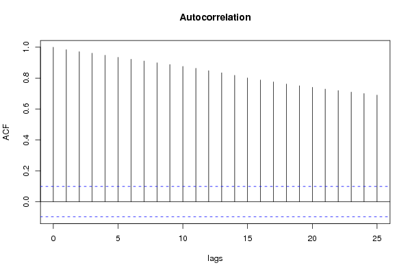
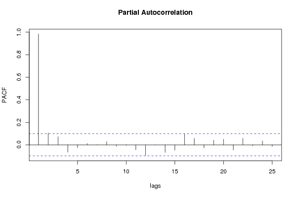
Title produced by software

(Partial) Autocorrelation Function

Date of computation

Wed, 17 Dec 2008 10:57:39 -0700

Cite this page as follows

Statistical Computations at FreeStatistics.org, Office for Research Development and Education, URL https://freestatistics.org/blog/index.php?v=date/2008/Dec/17/t1229536682z30n8yrpkjjg3sn.htm/, Retrieved Sun, 26 May 2024 16:40:31 +0000

Statistical Computations at FreeStatistics.org, Office for Research Development and Education, URL https://freestatistics.org/blog/index.php?pk=34454, Retrieved Sun, 26 May 2024 16:40:31 +0000

QR Codes:

Paste this QR Code to cite your computation.

Original text written by user:

IsPrivate?

No (this computation is public)

User-defined keywords

Estimated Impact

153

Family? (F = Feedback message, R = changed R code, M = changed R Module, P = changed Parameters, D = changed Data)

-       [(Partial) Autocorrelation Function] [VSA d=0; D=0] [2008-12-17 17:57:39] [d41d8cd98f00b204e9800998ecf8427e] [Current]

Feedback Forum

Post a new message

Dataseries X:

Download CSV

Histogram

Boxplots

Summary of computational transaction
Raw Input	view raw input (R code)
Raw Output	view raw output of R engine
Computing time	2 seconds
R Server	'Sir Ronald Aylmer Fisher' @ 193.190.124.24

\begin{tabular}{lllllllll}
\hline
Summary of computational transaction \tabularnewline
Raw Input & view raw input (R code)  \tabularnewline
Raw Output & view raw output of R engine  \tabularnewline
Computing time & 2 seconds \tabularnewline
R Server & 'Sir Ronald Aylmer Fisher' @ 193.190.124.24 \tabularnewline
\hline
\end{tabular}
%Source: https://freestatistics.org/blog/index.php?pk=34454&T=0

[TABLE]
[ROW][C]Summary of computational transaction[/C][/ROW]
[ROW][C]Raw Input[/C][C]view raw input (R code) [/C][/ROW]
[ROW][C]Raw Output[/C][C]view raw output of R engine [/C][/ROW]
[ROW][C]Computing time[/C][C]2 seconds[/C][/ROW]
[ROW][C]R Server[/C][C]'Sir Ronald Aylmer Fisher' @ 193.190.124.24[/C][/ROW]
[/TABLE]
Source: https://freestatistics.org/blog/index.php?pk=34454&T=0

Globally Unique Identifier (entire table): ba.freestatistics.org/blog/index.php?pk=34454&T=0

As an alternative you can also use a QR Code:

The GUIDs for individual cells are displayed in the table below:

Summary of computational transaction
Raw Input	view raw input (R code)
Raw Output	view raw output of R engine
Computing time	2 seconds
R Server	'Sir Ronald Aylmer Fisher' @ 193.190.124.24

Autocorrelation Function
Time lag k	ACF(k)	T-STAT	P-value
1	0.983802	19.5527	0
2	0.971251	19.3032	0
3	0.960806	19.0956	0
4	0.94794	18.8399	0
5	0.934823	18.5792	0
6	0.922704	18.3384	0
7	0.91057	18.0972	0
8	0.899334	17.8739	0
9	0.887726	17.6432	0
10	0.876127	17.4127	0
11	0.863496	17.1616	0
12	0.848382	16.8613	0
13	0.834158	16.5786	0
14	0.81815	16.2604	0
15	0.800889	15.9173	0
16	0.787566	15.6526	0
17	0.775497	15.4127	0
18	0.761773	15.1399	0
19	0.750329	14.9125	0
20	0.740647	14.7201	0
21	0.728924	14.4871	0
22	0.719312	14.296	0
23	0.709192	14.0949	0
24	0.699861	13.9095	0
25	0.689878	13.7111	0

\begin{tabular}{lllllllll}
\hline
Autocorrelation Function \tabularnewline
Time lag k & ACF(k) & T-STAT & P-value \tabularnewline
1 & 0.983802 & 19.5527 & 0 \tabularnewline
2 & 0.971251 & 19.3032 & 0 \tabularnewline
3 & 0.960806 & 19.0956 & 0 \tabularnewline
4 & 0.94794 & 18.8399 & 0 \tabularnewline
5 & 0.934823 & 18.5792 & 0 \tabularnewline
6 & 0.922704 & 18.3384 & 0 \tabularnewline
7 & 0.91057 & 18.0972 & 0 \tabularnewline
8 & 0.899334 & 17.8739 & 0 \tabularnewline
9 & 0.887726 & 17.6432 & 0 \tabularnewline
10 & 0.876127 & 17.4127 & 0 \tabularnewline
11 & 0.863496 & 17.1616 & 0 \tabularnewline
12 & 0.848382 & 16.8613 & 0 \tabularnewline
13 & 0.834158 & 16.5786 & 0 \tabularnewline
14 & 0.81815 & 16.2604 & 0 \tabularnewline
15 & 0.800889 & 15.9173 & 0 \tabularnewline
16 & 0.787566 & 15.6526 & 0 \tabularnewline
17 & 0.775497 & 15.4127 & 0 \tabularnewline
18 & 0.761773 & 15.1399 & 0 \tabularnewline
19 & 0.750329 & 14.9125 & 0 \tabularnewline
20 & 0.740647 & 14.7201 & 0 \tabularnewline
21 & 0.728924 & 14.4871 & 0 \tabularnewline
22 & 0.719312 & 14.296 & 0 \tabularnewline
23 & 0.709192 & 14.0949 & 0 \tabularnewline
24 & 0.699861 & 13.9095 & 0 \tabularnewline
25 & 0.689878 & 13.7111 & 0 \tabularnewline
\hline
\end{tabular}
%Source: https://freestatistics.org/blog/index.php?pk=34454&T=1

[TABLE]
[ROW][C]Autocorrelation Function[/C][/ROW]
[ROW][C]Time lag k[/C][C]ACF(k)[/C][C]T-STAT[/C][C]P-value[/C][/ROW]
[ROW][C]1[/C][C]0.983802[/C][C]19.5527[/C][C]0[/C][/ROW]
[ROW][C]2[/C][C]0.971251[/C][C]19.3032[/C][C]0[/C][/ROW]
[ROW][C]3[/C][C]0.960806[/C][C]19.0956[/C][C]0[/C][/ROW]
[ROW][C]4[/C][C]0.94794[/C][C]18.8399[/C][C]0[/C][/ROW]
[ROW][C]5[/C][C]0.934823[/C][C]18.5792[/C][C]0[/C][/ROW]
[ROW][C]6[/C][C]0.922704[/C][C]18.3384[/C][C]0[/C][/ROW]
[ROW][C]7[/C][C]0.91057[/C][C]18.0972[/C][C]0[/C][/ROW]
[ROW][C]8[/C][C]0.899334[/C][C]17.8739[/C][C]0[/C][/ROW]
[ROW][C]9[/C][C]0.887726[/C][C]17.6432[/C][C]0[/C][/ROW]
[ROW][C]10[/C][C]0.876127[/C][C]17.4127[/C][C]0[/C][/ROW]
[ROW][C]11[/C][C]0.863496[/C][C]17.1616[/C][C]0[/C][/ROW]
[ROW][C]12[/C][C]0.848382[/C][C]16.8613[/C][C]0[/C][/ROW]
[ROW][C]13[/C][C]0.834158[/C][C]16.5786[/C][C]0[/C][/ROW]
[ROW][C]14[/C][C]0.81815[/C][C]16.2604[/C][C]0[/C][/ROW]
[ROW][C]15[/C][C]0.800889[/C][C]15.9173[/C][C]0[/C][/ROW]
[ROW][C]16[/C][C]0.787566[/C][C]15.6526[/C][C]0[/C][/ROW]
[ROW][C]17[/C][C]0.775497[/C][C]15.4127[/C][C]0[/C][/ROW]
[ROW][C]18[/C][C]0.761773[/C][C]15.1399[/C][C]0[/C][/ROW]
[ROW][C]19[/C][C]0.750329[/C][C]14.9125[/C][C]0[/C][/ROW]
[ROW][C]20[/C][C]0.740647[/C][C]14.7201[/C][C]0[/C][/ROW]
[ROW][C]21[/C][C]0.728924[/C][C]14.4871[/C][C]0[/C][/ROW]
[ROW][C]22[/C][C]0.719312[/C][C]14.296[/C][C]0[/C][/ROW]
[ROW][C]23[/C][C]0.709192[/C][C]14.0949[/C][C]0[/C][/ROW]
[ROW][C]24[/C][C]0.699861[/C][C]13.9095[/C][C]0[/C][/ROW]
[ROW][C]25[/C][C]0.689878[/C][C]13.7111[/C][C]0[/C][/ROW]
[/TABLE]
Source: https://freestatistics.org/blog/index.php?pk=34454&T=1

Globally Unique Identifier (entire table): ba.freestatistics.org/blog/index.php?pk=34454&T=1

As an alternative you can also use a QR Code:

The GUIDs for individual cells are displayed in the table below:

Autocorrelation Function
Time lag k	ACF(k)	T-STAT	P-value
1	0.983802	19.5527	0
2	0.971251	19.3032	0
3	0.960806	19.0956	0
4	0.94794	18.8399	0
5	0.934823	18.5792	0
6	0.922704	18.3384	0
7	0.91057	18.0972	0
8	0.899334	17.8739	0
9	0.887726	17.6432	0
10	0.876127	17.4127	0
11	0.863496	17.1616	0
12	0.848382	16.8613	0
13	0.834158	16.5786	0
14	0.81815	16.2604	0
15	0.800889	15.9173	0
16	0.787566	15.6526	0
17	0.775497	15.4127	0
18	0.761773	15.1399	0
19	0.750329	14.9125	0
20	0.740647	14.7201	0
21	0.728924	14.4871	0
22	0.719312	14.296	0
23	0.709192	14.0949	0
24	0.699861	13.9095	0
25	0.689878	13.7111	0

Partial Autocorrelation Function
Time lag k	PACF(k)	T-STAT	P-value
1	0.983802	19.5527	0
2	0.10532	2.0932	0.018485
3	0.072644	1.4438	0.074798
4	-0.065042	-1.2927	0.098438
5	-0.025413	-0.5051	0.306895
6	0.012453	0.2475	0.402326
7	0.001903	0.0378	0.484926
8	0.02834	0.5632	0.286796
9	-0.013194	-0.2622	0.396644
10	-0.00547	-0.1087	0.45674
11	-0.043901	-0.8725	0.191729
12	-0.093275	-1.8538	0.032256
13	-0.001837	-0.0365	0.485444
14	-0.066856	-1.3287	0.092351
15	-0.047765	-0.9493	0.171523
16	0.097836	1.9444	0.026276
17	0.058478	1.1622	0.122922
18	-0.028238	-0.5612	0.28748
19	0.042639	0.8474	0.198632
20	0.050312	0.9999	0.158978
21	-0.045336	-0.901	0.184058
22	0.058858	1.1698	0.121398
23	-0.008265	-0.1643	0.434806
24	0.035856	0.7126	0.238247
25	-0.015348	-0.305	0.380251

\begin{tabular}{lllllllll}
\hline
Partial Autocorrelation Function \tabularnewline
Time lag k & PACF(k) & T-STAT & P-value \tabularnewline
1 & 0.983802 & 19.5527 & 0 \tabularnewline
2 & 0.10532 & 2.0932 & 0.018485 \tabularnewline
3 & 0.072644 & 1.4438 & 0.074798 \tabularnewline
4 & -0.065042 & -1.2927 & 0.098438 \tabularnewline
5 & -0.025413 & -0.5051 & 0.306895 \tabularnewline
6 & 0.012453 & 0.2475 & 0.402326 \tabularnewline
7 & 0.001903 & 0.0378 & 0.484926 \tabularnewline
8 & 0.02834 & 0.5632 & 0.286796 \tabularnewline
9 & -0.013194 & -0.2622 & 0.396644 \tabularnewline
10 & -0.00547 & -0.1087 & 0.45674 \tabularnewline
11 & -0.043901 & -0.8725 & 0.191729 \tabularnewline
12 & -0.093275 & -1.8538 & 0.032256 \tabularnewline
13 & -0.001837 & -0.0365 & 0.485444 \tabularnewline
14 & -0.066856 & -1.3287 & 0.092351 \tabularnewline
15 & -0.047765 & -0.9493 & 0.171523 \tabularnewline
16 & 0.097836 & 1.9444 & 0.026276 \tabularnewline
17 & 0.058478 & 1.1622 & 0.122922 \tabularnewline
18 & -0.028238 & -0.5612 & 0.28748 \tabularnewline
19 & 0.042639 & 0.8474 & 0.198632 \tabularnewline
20 & 0.050312 & 0.9999 & 0.158978 \tabularnewline
21 & -0.045336 & -0.901 & 0.184058 \tabularnewline
22 & 0.058858 & 1.1698 & 0.121398 \tabularnewline
23 & -0.008265 & -0.1643 & 0.434806 \tabularnewline
24 & 0.035856 & 0.7126 & 0.238247 \tabularnewline
25 & -0.015348 & -0.305 & 0.380251 \tabularnewline
\hline
\end{tabular}
%Source: https://freestatistics.org/blog/index.php?pk=34454&T=2

[TABLE]
[ROW][C]Partial Autocorrelation Function[/C][/ROW]
[ROW][C]Time lag k[/C][C]PACF(k)[/C][C]T-STAT[/C][C]P-value[/C][/ROW]
[ROW][C]1[/C][C]0.983802[/C][C]19.5527[/C][C]0[/C][/ROW]
[ROW][C]2[/C][C]0.10532[/C][C]2.0932[/C][C]0.018485[/C][/ROW]
[ROW][C]3[/C][C]0.072644[/C][C]1.4438[/C][C]0.074798[/C][/ROW]
[ROW][C]4[/C][C]-0.065042[/C][C]-1.2927[/C][C]0.098438[/C][/ROW]
[ROW][C]5[/C][C]-0.025413[/C][C]-0.5051[/C][C]0.306895[/C][/ROW]
[ROW][C]6[/C][C]0.012453[/C][C]0.2475[/C][C]0.402326[/C][/ROW]
[ROW][C]7[/C][C]0.001903[/C][C]0.0378[/C][C]0.484926[/C][/ROW]
[ROW][C]8[/C][C]0.02834[/C][C]0.5632[/C][C]0.286796[/C][/ROW]
[ROW][C]9[/C][C]-0.013194[/C][C]-0.2622[/C][C]0.396644[/C][/ROW]
[ROW][C]10[/C][C]-0.00547[/C][C]-0.1087[/C][C]0.45674[/C][/ROW]
[ROW][C]11[/C][C]-0.043901[/C][C]-0.8725[/C][C]0.191729[/C][/ROW]
[ROW][C]12[/C][C]-0.093275[/C][C]-1.8538[/C][C]0.032256[/C][/ROW]
[ROW][C]13[/C][C]-0.001837[/C][C]-0.0365[/C][C]0.485444[/C][/ROW]
[ROW][C]14[/C][C]-0.066856[/C][C]-1.3287[/C][C]0.092351[/C][/ROW]
[ROW][C]15[/C][C]-0.047765[/C][C]-0.9493[/C][C]0.171523[/C][/ROW]
[ROW][C]16[/C][C]0.097836[/C][C]1.9444[/C][C]0.026276[/C][/ROW]
[ROW][C]17[/C][C]0.058478[/C][C]1.1622[/C][C]0.122922[/C][/ROW]
[ROW][C]18[/C][C]-0.028238[/C][C]-0.5612[/C][C]0.28748[/C][/ROW]
[ROW][C]19[/C][C]0.042639[/C][C]0.8474[/C][C]0.198632[/C][/ROW]
[ROW][C]20[/C][C]0.050312[/C][C]0.9999[/C][C]0.158978[/C][/ROW]
[ROW][C]21[/C][C]-0.045336[/C][C]-0.901[/C][C]0.184058[/C][/ROW]
[ROW][C]22[/C][C]0.058858[/C][C]1.1698[/C][C]0.121398[/C][/ROW]
[ROW][C]23[/C][C]-0.008265[/C][C]-0.1643[/C][C]0.434806[/C][/ROW]
[ROW][C]24[/C][C]0.035856[/C][C]0.7126[/C][C]0.238247[/C][/ROW]
[ROW][C]25[/C][C]-0.015348[/C][C]-0.305[/C][C]0.380251[/C][/ROW]
[/TABLE]
Source: https://freestatistics.org/blog/index.php?pk=34454&T=2

Globally Unique Identifier (entire table): ba.freestatistics.org/blog/index.php?pk=34454&T=2

As an alternative you can also use a QR Code:

The GUIDs for individual cells are displayed in the table below:

Partial Autocorrelation Function
Time lag k	PACF(k)	T-STAT	P-value
1	0.983802	19.5527	0
2	0.10532	2.0932	0.018485
3	0.072644	1.4438	0.074798
4	-0.065042	-1.2927	0.098438
5	-0.025413	-0.5051	0.306895
6	0.012453	0.2475	0.402326
7	0.001903	0.0378	0.484926
8	0.02834	0.5632	0.286796
9	-0.013194	-0.2622	0.396644
10	-0.00547	-0.1087	0.45674
11	-0.043901	-0.8725	0.191729
12	-0.093275	-1.8538	0.032256
13	-0.001837	-0.0365	0.485444
14	-0.066856	-1.3287	0.092351
15	-0.047765	-0.9493	0.171523
16	0.097836	1.9444	0.026276
17	0.058478	1.1622	0.122922
18	-0.028238	-0.5612	0.28748
19	0.042639	0.8474	0.198632
20	0.050312	0.9999	0.158978
21	-0.045336	-0.901	0.184058
22	0.058858	1.1698	0.121398
23	-0.008265	-0.1643	0.434806
24	0.035856	0.7126	0.238247
25	-0.015348	-0.305	0.380251

Figure 1

PNG link

Postscript link

PDF link

Figure 2

PNG link

Postscript link

PDF link

Parameters (Session):

par1 = Default ; par2 = 1 ; par3 = 0 ; par4 = 0 ; par5 = 1 ;

Parameters (R input):

par1 = Default ; par2 = 1 ; par3 = 0 ; par4 = 0 ; par5 = 1 ;

R code (references can be found in the software module):

if (par1 == 'Default') {
par1 = 10*log10(length(x))
} else {
par1 <- as.numeric(par1)
}
par2 <- as.numeric(par2)
par3 <- as.numeric(par3)
par4 <- as.numeric(par4)
par5 <- as.numeric(par5)
if (par2 == 0) {
x <- log(x)
} else {
x <- (x ^ par2 - 1) / par2
}
if (par3 > 0) x <- diff(x,lag=1,difference=par3)
if (par4 > 0) x <- diff(x,lag=par5,difference=par4)
bitmap(file='pic1.png')
racf <- acf(x,par1,main='Autocorrelation',xlab='lags',ylab='ACF')
dev.off()
bitmap(file='pic2.png')
rpacf <- pacf(x,par1,main='Partial Autocorrelation',xlab='lags',ylab='PACF')
dev.off()
(myacf <- c(racf$acf))
(mypacf <- c(rpacf$acf))
lengthx <- length(x)
sqrtn <- sqrt(lengthx)
load(file='createtable')
a<-table.start()
a<-table.row.start(a)
a<-table.element(a,'Autocorrelation Function',4,TRUE)
a<-table.row.end(a)
a<-table.row.start(a)
a<-table.element(a,'Time lag k',header=TRUE)
a<-table.element(a,hyperlink('basics.htm','ACF(k)','click here for more information about the Autocorrelation Function'),header=TRUE)
a<-table.element(a,'T-STAT',header=TRUE)
a<-table.element(a,'P-value',header=TRUE)
a<-table.row.end(a)
for (i in 2:(par1+1)) {
a<-table.row.start(a)
a<-table.element(a,i-1,header=TRUE)
a<-table.element(a,round(myacf[i],6))
mytstat <- myacf[i]*sqrtn
a<-table.element(a,round(mytstat,4))
a<-table.element(a,round(1-pt(abs(mytstat),lengthx),6))
a<-table.row.end(a)
}
a<-table.end(a)
table.save(a,file='mytable.tab')
a<-table.start()
a<-table.row.start(a)
a<-table.element(a,'Partial Autocorrelation Function',4,TRUE)
a<-table.row.end(a)
a<-table.row.start(a)
a<-table.element(a,'Time lag k',header=TRUE)
a<-table.element(a,hyperlink('basics.htm','PACF(k)','click here for more information about the Partial Autocorrelation Function'),header=TRUE)
a<-table.element(a,'T-STAT',header=TRUE)
a<-table.element(a,'P-value',header=TRUE)
a<-table.row.end(a)
for (i in 1:par1) {
a<-table.row.start(a)
a<-table.element(a,i,header=TRUE)
a<-table.element(a,round(mypacf[i],6))
mytstat <- mypacf[i]*sqrtn
a<-table.element(a,round(mytstat,4))
a<-table.element(a,round(1-pt(abs(mytstat),lengthx),6))
a<-table.row.end(a)
}
a<-table.end(a)
table.save(a,file='mytable1.tab')

Free Statistics

Description of Statistical Computation

Tree of Dependent Computations

Dataset

Tables (Output of Computation)

Figures (Output of Computation)

Input Parameters & R Code