Free Statistics
of Irreproducible Research!
Description of Statistical Computation | |||||||||||||||||||||||||||||||||||||||||||||||||||||||||||||||||||||||||||||||||||||||||||||||||||||||||||||||||||||||||||||||||||||||||||||||||||||||||||||||||
|---|---|---|---|---|---|---|---|---|---|---|---|---|---|---|---|---|---|---|---|---|---|---|---|---|---|---|---|---|---|---|---|---|---|---|---|---|---|---|---|---|---|---|---|---|---|---|---|---|---|---|---|---|---|---|---|---|---|---|---|---|---|---|---|---|---|---|---|---|---|---|---|---|---|---|---|---|---|---|---|---|---|---|---|---|---|---|---|---|---|---|---|---|---|---|---|---|---|---|---|---|---|---|---|---|---|---|---|---|---|---|---|---|---|---|---|---|---|---|---|---|---|---|---|---|---|---|---|---|---|---|---|---|---|---|---|---|---|---|---|---|---|---|---|---|---|---|---|---|---|---|---|---|---|---|---|---|---|---|---|---|---|
| Author's title | |||||||||||||||||||||||||||||||||||||||||||||||||||||||||||||||||||||||||||||||||||||||||||||||||||||||||||||||||||||||||||||||||||||||||||||||||||||||||||||||||
| Author | *The author of this computation has been verified* | ||||||||||||||||||||||||||||||||||||||||||||||||||||||||||||||||||||||||||||||||||||||||||||||||||||||||||||||||||||||||||||||||||||||||||||||||||||||||||||||||
| R Software Module | rwasp_smp.wasp | ||||||||||||||||||||||||||||||||||||||||||||||||||||||||||||||||||||||||||||||||||||||||||||||||||||||||||||||||||||||||||||||||||||||||||||||||||||||||||||||||
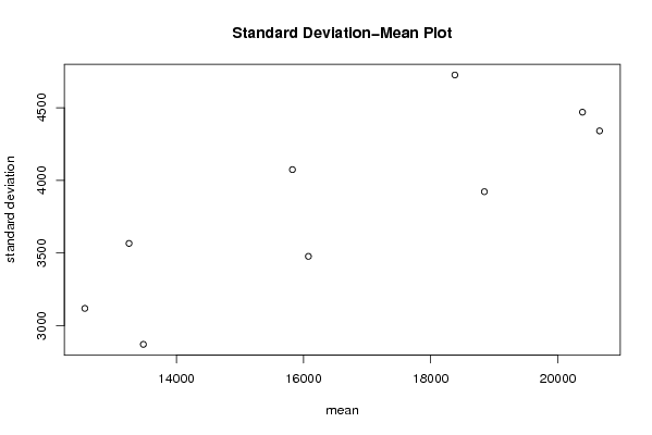
| Title produced by software | Standard Deviation-Mean Plot | ||||||||||||||||||||||||||||||||||||||||||||||||||||||||||||||||||||||||||||||||||||||||||||||||||||||||||||||||||||||||||||||||||||||||||||||||||||||||||||||||
| Date of computation | Mon, 15 Dec 2008 15:25:20 -0700 | ||||||||||||||||||||||||||||||||||||||||||||||||||||||||||||||||||||||||||||||||||||||||||||||||||||||||||||||||||||||||||||||||||||||||||||||||||||||||||||||||
| Cite this page as follows | Statistical Computations at FreeStatistics.org, Office for Research Development and Education, URL https://freestatistics.org/blog/index.php?v=date/2008/Dec/15/t1229379970cfg5erjmmzxwtcs.htm/, Retrieved Sat, 06 Jun 2026 07:31:55 +0000 | ||||||||||||||||||||||||||||||||||||||||||||||||||||||||||||||||||||||||||||||||||||||||||||||||||||||||||||||||||||||||||||||||||||||||||||||||||||||||||||||||
| Statistical Computations at FreeStatistics.org, Office for Research Development and Education, URL https://freestatistics.org/blog/index.php?pk=33836, Retrieved Sat, 06 Jun 2026 07:31:55 +0000 | |||||||||||||||||||||||||||||||||||||||||||||||||||||||||||||||||||||||||||||||||||||||||||||||||||||||||||||||||||||||||||||||||||||||||||||||||||||||||||||||||
| QR Codes: | |||||||||||||||||||||||||||||||||||||||||||||||||||||||||||||||||||||||||||||||||||||||||||||||||||||||||||||||||||||||||||||||||||||||||||||||||||||||||||||||||
|
| |||||||||||||||||||||||||||||||||||||||||||||||||||||||||||||||||||||||||||||||||||||||||||||||||||||||||||||||||||||||||||||||||||||||||||||||||||||||||||||||||
| Original text written by user: | |||||||||||||||||||||||||||||||||||||||||||||||||||||||||||||||||||||||||||||||||||||||||||||||||||||||||||||||||||||||||||||||||||||||||||||||||||||||||||||||||
| IsPrivate? | No (this computation is public) | ||||||||||||||||||||||||||||||||||||||||||||||||||||||||||||||||||||||||||||||||||||||||||||||||||||||||||||||||||||||||||||||||||||||||||||||||||||||||||||||||
| User-defined keywords | |||||||||||||||||||||||||||||||||||||||||||||||||||||||||||||||||||||||||||||||||||||||||||||||||||||||||||||||||||||||||||||||||||||||||||||||||||||||||||||||||
| Estimated Impact | 536 | ||||||||||||||||||||||||||||||||||||||||||||||||||||||||||||||||||||||||||||||||||||||||||||||||||||||||||||||||||||||||||||||||||||||||||||||||||||||||||||||||
Tree of Dependent Computations | |||||||||||||||||||||||||||||||||||||||||||||||||||||||||||||||||||||||||||||||||||||||||||||||||||||||||||||||||||||||||||||||||||||||||||||||||||||||||||||||||
| Family? (F = Feedback message, R = changed R code, M = changed R Module, P = changed Parameters, D = changed Data) | |||||||||||||||||||||||||||||||||||||||||||||||||||||||||||||||||||||||||||||||||||||||||||||||||||||||||||||||||||||||||||||||||||||||||||||||||||||||||||||||||
| - [Standard Deviation-Mean Plot] [SMP prof bach] [2008-12-15 22:25:20] [21d7d81e7693ad6dde5aadefb1046611] [Current] - RM [Variance Reduction Matrix] [VRM prof bach] [2008-12-15 22:31:00] [bc937651ef42bf891200cf0e0edc7238] - RMP [(Partial) Autocorrelation Function] [ARIMA Prof bach A...] [2008-12-15 22:38:57] [bc937651ef42bf891200cf0e0edc7238] - P [(Partial) Autocorrelation Function] [ARIMA ACF prof ba...] [2008-12-15 22:41:53] [bc937651ef42bf891200cf0e0edc7238] - P [(Partial) Autocorrelation Function] [ARIMA ACF prof ba...] [2008-12-15 22:44:07] [bc937651ef42bf891200cf0e0edc7238] - P [(Partial) Autocorrelation Function] [ARIMA ACF prof ba...] [2008-12-15 22:46:08] [bc937651ef42bf891200cf0e0edc7238] - P [(Partial) Autocorrelation Function] [acf prof bach L =...] [2008-12-19 15:35:04] [bc937651ef42bf891200cf0e0edc7238] - P [(Partial) Autocorrelation Function] [acf prof bach lam...] [2008-12-19 15:40:07] [bc937651ef42bf891200cf0e0edc7238] - P [(Partial) Autocorrelation Function] [acf prof bach lam...] [2008-12-19 15:40:07] [bc937651ef42bf891200cf0e0edc7238] - P [(Partial) Autocorrelation Function] [acf lambda = 1,1,1] [2008-12-19 15:45:45] [bc937651ef42bf891200cf0e0edc7238] - MPD [(Partial) Autocorrelation Function] [ACF bij d=0 en D=0] [2010-12-17 13:29:13] [616fb52b46273b7e6805de1e68b3a688] - P [(Partial) Autocorrelation Function] [ACF bij d=0 en D=1] [2010-12-17 13:34:11] [616fb52b46273b7e6805de1e68b3a688] - P [(Partial) Autocorrelation Function] [ACF bij d=1 en D=1] [2010-12-17 13:51:58] [616fb52b46273b7e6805de1e68b3a688] - MPD [(Partial) Autocorrelation Function] [] [2010-12-24 12:03:15] [4dfa50539945b119a90a7606969443b9] - MPD [(Partial) Autocorrelation Function] [] [2010-12-24 12:12:12] [4dfa50539945b119a90a7606969443b9] - RMP [ARIMA Backward Selection] [Arima backward se...] [2008-12-19 17:26:16] [bc937651ef42bf891200cf0e0edc7238] - RMP [ARIMA Forecasting] [ARIMA forecast pr...] [2008-12-20 11:34:44] [bc937651ef42bf891200cf0e0edc7238] - MPD [ARIMA Forecasting] [] [2010-12-21 19:37:30] [94f4aa1c01e87d8321fffb341ed4df07] - D [ARIMA Forecasting] [] [2010-12-22 16:40:18] [94f4aa1c01e87d8321fffb341ed4df07] - MPD [ARIMA Forecasting] [ARIMA Forecasting] [2010-12-22 13:25:50] [616fb52b46273b7e6805de1e68b3a688] - D [ARIMA Forecasting] [ARIMA Forecasting] [2010-12-24 15:04:34] [616fb52b46273b7e6805de1e68b3a688] - RMPD [ARIMA Forecasting] [] [2010-12-24 13:59:54] [4dfa50539945b119a90a7606969443b9] - PD [ARIMA Forecasting] [] [2010-12-26 10:14:56] [4dfa50539945b119a90a7606969443b9] - RMP [ARIMA Forecasting] [ARIMA forecast pr...] [2008-12-20 11:40:03] [bc937651ef42bf891200cf0e0edc7238] - P [ARIMA Forecasting] [ARIMA forecast pr...] [2008-12-20 13:00:09] [bc937651ef42bf891200cf0e0edc7238] - P [ARIMA Forecasting] [ARIMA voorspellin...] [2008-12-20 13:17:10] [bc937651ef42bf891200cf0e0edc7238] - M D [ARIMA Backward Selection] [] [2010-12-21 17:53:23] [94f4aa1c01e87d8321fffb341ed4df07] - MPD [ARIMA Backward Selection] [] [2010-12-21 19:17:29] [94f4aa1c01e87d8321fffb341ed4df07] - MPD [ARIMA Backward Selection] [] [2010-12-24 13:46:46] [4dfa50539945b119a90a7606969443b9] - MPD [ARIMA Backward Selection] [Paper Statistiek] [2010-12-28 15:46:48] [82c18f3ebe9df70882495121eb816e07] - MP [ARIMA Backward Selection] [Paper Statistiek] [2010-12-28 16:09:56] [82c18f3ebe9df70882495121eb816e07] - RMPD [ARIMA Backward Selection] [ARIMA Backward Se...] [2010-12-28 18:28:51] [74be16979710d4c4e7c6647856088456] - MPD [(Partial) Autocorrelation Function] [] [2010-12-20 16:16:49] [94f4aa1c01e87d8321fffb341ed4df07] - MPD [(Partial) Autocorrelation Function] [b-r0245787] [2010-12-22 14:53:44] [ebb35fb07def4d07c0eb7ec8d2fd3b0e] - [(Partial) Autocorrelation Function] [b-r0245095] [2010-12-22 14:58:29] [ec8d68d52c1e9c5e97bb689b42436a8c] - PD [(Partial) Autocorrelation Function] [b-r0245095] [2010-12-22 15:32:51] [ec8d68d52c1e9c5e97bb689b42436a8c] - PD [(Partial) Autocorrelation Function] [b-r0245787] [2010-12-22 15:30:39] [ebb35fb07def4d07c0eb7ec8d2fd3b0e] - MPD [(Partial) Autocorrelation Function] [] [2010-12-24 12:53:41] [4dfa50539945b119a90a7606969443b9] - MPD [(Partial) Autocorrelation Function] [] [2010-12-28 12:28:43] [c6813a60da787bb62b5d86150b8926dd] - R P [(Partial) Autocorrelation Function] [Deel 4: ARIMA bac...] [2012-12-13 15:17:46] [b4e5b8b5af0253f45dc68b47bb41cf13] - RMPD [(Partial) Autocorrelation Function] [Autocorrelation] [2010-12-28 16:20:44] [74be16979710d4c4e7c6647856088456] - RMPD [ARIMA Backward Selection] [arima-model] [2010-12-29 22:10:14] [5a05da414fd67612c3b80d44effe0727] - RMPD [] [Standard Deviatio...] [-0001-11-30 00:00:00] [616fb52b46273b7e6805de1e68b3a688] | |||||||||||||||||||||||||||||||||||||||||||||||||||||||||||||||||||||||||||||||||||||||||||||||||||||||||||||||||||||||||||||||||||||||||||||||||||||||||||||||||
| Feedback Forum | |||||||||||||||||||||||||||||||||||||||||||||||||||||||||||||||||||||||||||||||||||||||||||||||||||||||||||||||||||||||||||||||||||||||||||||||||||||||||||||||||
Post a new message | |||||||||||||||||||||||||||||||||||||||||||||||||||||||||||||||||||||||||||||||||||||||||||||||||||||||||||||||||||||||||||||||||||||||||||||||||||||||||||||||||
Dataset | |||||||||||||||||||||||||||||||||||||||||||||||||||||||||||||||||||||||||||||||||||||||||||||||||||||||||||||||||||||||||||||||||||||||||||||||||||||||||||||||||
| Dataseries X: | |||||||||||||||||||||||||||||||||||||||||||||||||||||||||||||||||||||||||||||||||||||||||||||||||||||||||||||||||||||||||||||||||||||||||||||||||||||||||||||||||
13363 12530 11420 10948 10173 10602 16094 19631 17140 14345 12632 12894 11808 10673 9939 9890 9283 10131 15864 19283 16203 13919 11937 11795 11268 10522 9929 9725 9372 10068 16230 19115 18351 16265 14103 14115 13327 12618 12129 11775 11493 12470 20792 22337 21325 18581 16475 16581 15745 14453 13712 13766 13336 15346 24446 26178 24628 21282 18850 18822 18060 17536 16417 15842 15188 16905 25430 27962 26607 23364 20827 20506 19181 18016 17354 16256 15770 17538 26899 28915 25247 22856 19980 19856 16994 16839 15618 15883 15513 17106 25272 26731 22891 19583 16939 16757 15435 14786 13680 13208 12707 14277 22436 23229 18241 16145 13994 14780 13100 12329 12463 11532 10784 13106 19491 20418 16094 14491 13067 | |||||||||||||||||||||||||||||||||||||||||||||||||||||||||||||||||||||||||||||||||||||||||||||||||||||||||||||||||||||||||||||||||||||||||||||||||||||||||||||||||
Tables (Output of Computation) | |||||||||||||||||||||||||||||||||||||||||||||||||||||||||||||||||||||||||||||||||||||||||||||||||||||||||||||||||||||||||||||||||||||||||||||||||||||||||||||||||
| |||||||||||||||||||||||||||||||||||||||||||||||||||||||||||||||||||||||||||||||||||||||||||||||||||||||||||||||||||||||||||||||||||||||||||||||||||||||||||||||||
Figures (Output of Computation) | |||||||||||||||||||||||||||||||||||||||||||||||||||||||||||||||||||||||||||||||||||||||||||||||||||||||||||||||||||||||||||||||||||||||||||||||||||||||||||||||||
Input Parameters & R Code | |||||||||||||||||||||||||||||||||||||||||||||||||||||||||||||||||||||||||||||||||||||||||||||||||||||||||||||||||||||||||||||||||||||||||||||||||||||||||||||||||
| Parameters (Session): | |||||||||||||||||||||||||||||||||||||||||||||||||||||||||||||||||||||||||||||||||||||||||||||||||||||||||||||||||||||||||||||||||||||||||||||||||||||||||||||||||
| par1 = 12 ; | |||||||||||||||||||||||||||||||||||||||||||||||||||||||||||||||||||||||||||||||||||||||||||||||||||||||||||||||||||||||||||||||||||||||||||||||||||||||||||||||||
| Parameters (R input): | |||||||||||||||||||||||||||||||||||||||||||||||||||||||||||||||||||||||||||||||||||||||||||||||||||||||||||||||||||||||||||||||||||||||||||||||||||||||||||||||||
| par1 = 12 ; | |||||||||||||||||||||||||||||||||||||||||||||||||||||||||||||||||||||||||||||||||||||||||||||||||||||||||||||||||||||||||||||||||||||||||||||||||||||||||||||||||
| R code (references can be found in the software module): | |||||||||||||||||||||||||||||||||||||||||||||||||||||||||||||||||||||||||||||||||||||||||||||||||||||||||||||||||||||||||||||||||||||||||||||||||||||||||||||||||
par1 <- as.numeric(par1) | |||||||||||||||||||||||||||||||||||||||||||||||||||||||||||||||||||||||||||||||||||||||||||||||||||||||||||||||||||||||||||||||||||||||||||||||||||||||||||||||||