Free Statistics
of Irreproducible Research!
Description of Statistical Computation | |||||||||||||||||||||||||||||||||||||||||||||||||||||
|---|---|---|---|---|---|---|---|---|---|---|---|---|---|---|---|---|---|---|---|---|---|---|---|---|---|---|---|---|---|---|---|---|---|---|---|---|---|---|---|---|---|---|---|---|---|---|---|---|---|---|---|---|---|
| Author's title | |||||||||||||||||||||||||||||||||||||||||||||||||||||
| Author | *Unverified author* | ||||||||||||||||||||||||||||||||||||||||||||||||||||
| R Software Module | rwasp_edauni.wasp | ||||||||||||||||||||||||||||||||||||||||||||||||||||
| Title produced by software | Univariate Explorative Data Analysis | ||||||||||||||||||||||||||||||||||||||||||||||||||||
| Date of computation | Sat, 13 Dec 2008 03:22:17 -0700 | ||||||||||||||||||||||||||||||||||||||||||||||||||||
| Cite this page as follows | Statistical Computations at FreeStatistics.org, Office for Research Development and Education, URL https://freestatistics.org/blog/index.php?v=date/2008/Dec/13/t122916382303osgt9yvutt69y.htm/, Retrieved Thu, 22 Jan 2026 11:06:51 +0000 | ||||||||||||||||||||||||||||||||||||||||||||||||||||
| Statistical Computations at FreeStatistics.org, Office for Research Development and Education, URL https://freestatistics.org/blog/index.php?pk=32943, Retrieved Thu, 22 Jan 2026 11:06:51 +0000 | |||||||||||||||||||||||||||||||||||||||||||||||||||||
| QR Codes: | |||||||||||||||||||||||||||||||||||||||||||||||||||||
|
| |||||||||||||||||||||||||||||||||||||||||||||||||||||
| Original text written by user: | |||||||||||||||||||||||||||||||||||||||||||||||||||||
| IsPrivate? | No (this computation is public) | ||||||||||||||||||||||||||||||||||||||||||||||||||||
| User-defined keywords | |||||||||||||||||||||||||||||||||||||||||||||||||||||
| Estimated Impact | 474 | ||||||||||||||||||||||||||||||||||||||||||||||||||||
Tree of Dependent Computations | |||||||||||||||||||||||||||||||||||||||||||||||||||||
| Family? (F = Feedback message, R = changed R code, M = changed R Module, P = changed Parameters, D = changed Data) | |||||||||||||||||||||||||||||||||||||||||||||||||||||
| - [Univariate Explorative Data Analysis] [bel20 univariate ...] [2008-12-10 17:19:38] [74be16979710d4c4e7c6647856088456] - D [Univariate Explorative Data Analysis] [univariate EDA do...] [2008-12-13 10:22:17] [c8dc05b1cdf5010d9a4f2d773adefb82] [Current] | |||||||||||||||||||||||||||||||||||||||||||||||||||||
| Feedback Forum | |||||||||||||||||||||||||||||||||||||||||||||||||||||
Post a new message | |||||||||||||||||||||||||||||||||||||||||||||||||||||
Dataset | |||||||||||||||||||||||||||||||||||||||||||||||||||||
| Dataseries X: | |||||||||||||||||||||||||||||||||||||||||||||||||||||
9005,73 9018,68 9349,44 9327,78 9753,63 10443,5 10853,87 10704,02 11052,23 10935,47 10714,03 10394,48 10817,9 11251,2 11281,26 10539,68 10483,39 10947,43 10580,27 10582,92 10654,41 11014,51 10967,87 10433,56 10665,78 10666,71 10682,74 10777,22 10052,6 10213,97 10546,82 10767,2 10444,5 10314,68 9042,56 9220,75 9721,84 9978,53 9923,81 9892,56 10500,98 10179,35 10080,48 9492,44 8616,49 8685,4 8160,67 8048,1 8641,21 8526,63 8474,21 7916,13 7977,64 8334,59 8623,36 9098,03 9154,34 9284,73 9492,49 9682,35 9762,12 10124,63 10540,05 10601,61 10323,73 10418,4 10092,96 10364,91 10152,09 10032,8 10204,59 10001,6 10411,75 10673,38 10539,51 10723,78 10682,06 10283,19 10377,18 10486,64 10545,38 10554,27 10532,54 10324,31 10695,25 10827,81 10872,48 10971,19 11145,65 11234,68 11333,88 10997,97 11036,89 11257,35 11533,59 11963,12 12185,15 12377,62 12512,89 12631,48 12268,53 12754,8 13407,75 13480,21 13673,28 13239,71 13557,69 13901,28 13200,58 13406,97 12538,12 12419,57 12193,88 12656,63 12812,48 12056,67 11322,38 11530,75 11114,08 9181,73 8614,55 | |||||||||||||||||||||||||||||||||||||||||||||||||||||
Tables (Output of Computation) | |||||||||||||||||||||||||||||||||||||||||||||||||||||
| |||||||||||||||||||||||||||||||||||||||||||||||||||||
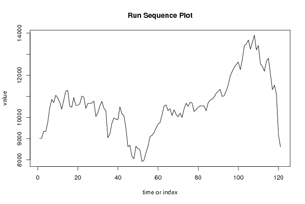
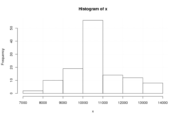
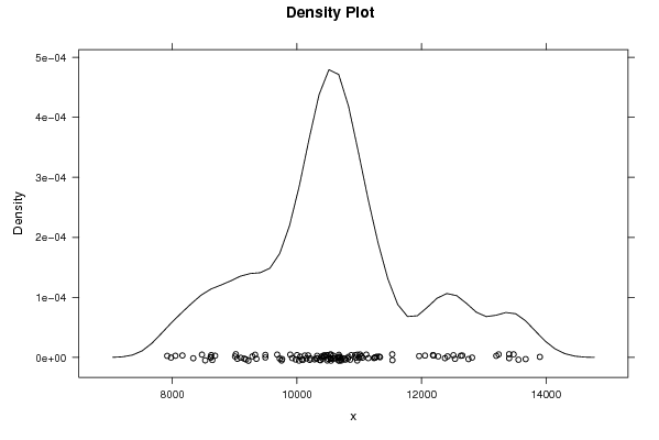
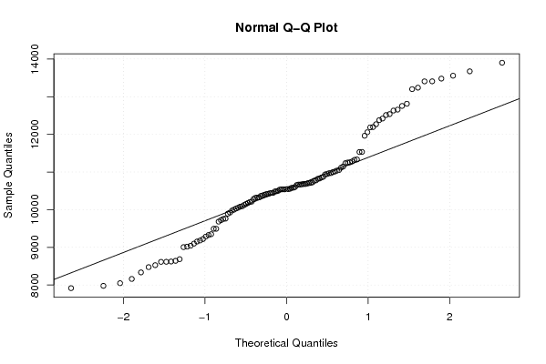
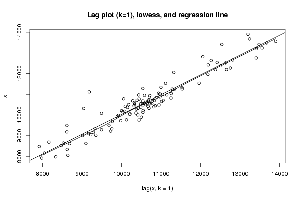
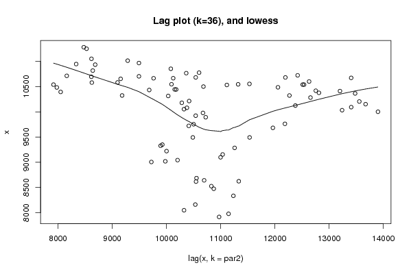
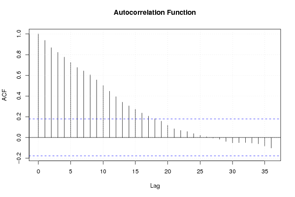
Figures (Output of Computation) | |||||||||||||||||||||||||||||||||||||||||||||||||||||
Input Parameters & R Code | |||||||||||||||||||||||||||||||||||||||||||||||||||||
| Parameters (Session): | |||||||||||||||||||||||||||||||||||||||||||||||||||||
| par1 = 0 ; par2 = 36 ; | |||||||||||||||||||||||||||||||||||||||||||||||||||||
| Parameters (R input): | |||||||||||||||||||||||||||||||||||||||||||||||||||||
| par1 = 0 ; par2 = 36 ; | |||||||||||||||||||||||||||||||||||||||||||||||||||||
| R code (references can be found in the software module): | |||||||||||||||||||||||||||||||||||||||||||||||||||||
par1 <- as.numeric(par1) | |||||||||||||||||||||||||||||||||||||||||||||||||||||