Free Statistics
of Irreproducible Research!
Description of Statistical Computation | |||||||||||||||||||||||||||||||||||||
|---|---|---|---|---|---|---|---|---|---|---|---|---|---|---|---|---|---|---|---|---|---|---|---|---|---|---|---|---|---|---|---|---|---|---|---|---|---|
| Author's title | |||||||||||||||||||||||||||||||||||||
| Author | *The author of this computation has been verified* | ||||||||||||||||||||||||||||||||||||
| R Software Module | rwasp_boxcoxnorm.wasp | ||||||||||||||||||||||||||||||||||||
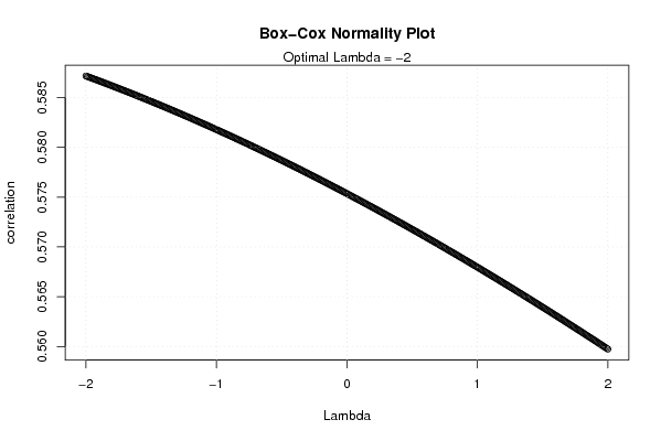
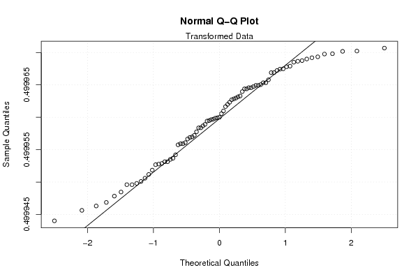
| Title produced by software | Box-Cox Normality Plot | ||||||||||||||||||||||||||||||||||||
| Date of computation | Thu, 11 Dec 2008 08:53:23 -0700 | ||||||||||||||||||||||||||||||||||||
| Cite this page as follows | Statistical Computations at FreeStatistics.org, Office for Research Development and Education, URL https://freestatistics.org/blog/index.php?v=date/2008/Dec/11/t1229010949ilglzqexkajjz7z.htm/, Retrieved Sat, 25 May 2024 03:13:54 +0000 | ||||||||||||||||||||||||||||||||||||
| Statistical Computations at FreeStatistics.org, Office for Research Development and Education, URL https://freestatistics.org/blog/index.php?pk=32321, Retrieved Sat, 25 May 2024 03:13:54 +0000 | |||||||||||||||||||||||||||||||||||||
| QR Codes: | |||||||||||||||||||||||||||||||||||||
|
| |||||||||||||||||||||||||||||||||||||
| Original text written by user: | |||||||||||||||||||||||||||||||||||||
| IsPrivate? | No (this computation is public) | ||||||||||||||||||||||||||||||||||||
| User-defined keywords | |||||||||||||||||||||||||||||||||||||
| Estimated Impact | 182 | ||||||||||||||||||||||||||||||||||||
Tree of Dependent Computations | |||||||||||||||||||||||||||||||||||||
| Family? (F = Feedback message, R = changed R code, M = changed R Module, P = changed Parameters, D = changed Data) | |||||||||||||||||||||||||||||||||||||
| - [Standard Deviation-Mean Plot] [Standard Deviatio...] [2008-12-11 14:19:03] [b518240a1c80d4f939bf8b3e34f77cec] - RMPD [Box-Cox Normality Plot] [Box-Cox Normality...] [2008-12-11 15:53:23] [6aa66640011d9b98524a5838bcf7301d] [Current] | |||||||||||||||||||||||||||||||||||||
| Feedback Forum | |||||||||||||||||||||||||||||||||||||
Post a new message | |||||||||||||||||||||||||||||||||||||
Dataset | |||||||||||||||||||||||||||||||||||||
| Dataseries X: | |||||||||||||||||||||||||||||||||||||
98,5 97,0 103,3 99,6 100,1 102,9 95,9 94,5 107,4 116,0 102,8 99,8 109,6 103,0 111,6 106,3 97,9 108,8 103,9 101,2 122,9 123,9 111,7 120,9 99,6 103,3 119,4 106,5 101,9 124,6 106,5 107,8 127,4 120,1 118,5 127,7 107,7 104,5 118,8 110,3 109,6 119,1 96,5 106,7 126,3 116,2 118,8 115,2 110,0 111,4 129,6 108,1 117,8 122,9 100,6 111,8 127,0 128,6 124,8 118,5 114,7 112,6 128,7 111,0 115,8 126,0 111,1 113,2 120,1 130,6 124,0 119,4 116,7 116,5 119,6 126,5 111,3 123,5 114,2 103,7 129,5 | |||||||||||||||||||||||||||||||||||||
Tables (Output of Computation) | |||||||||||||||||||||||||||||||||||||
| |||||||||||||||||||||||||||||||||||||
Figures (Output of Computation) | |||||||||||||||||||||||||||||||||||||
Input Parameters & R Code | |||||||||||||||||||||||||||||||||||||
| Parameters (Session): | |||||||||||||||||||||||||||||||||||||
| Parameters (R input): | |||||||||||||||||||||||||||||||||||||
| R code (references can be found in the software module): | |||||||||||||||||||||||||||||||||||||
n <- length(x) | |||||||||||||||||||||||||||||||||||||