Repository of Reproducible Computations

Free Statistics

of Irreproducible Research!

Author's title

Author

*Unverified author*

R Software Module

rwasp_autocorrelation.wasp

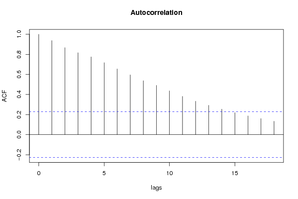
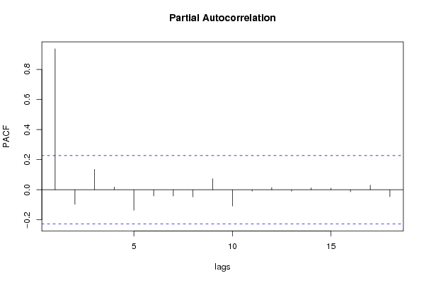
Title produced by software

(Partial) Autocorrelation Function

Date of computation

Sat, 06 Dec 2008 09:30:23 -0700

Cite this page as follows

Statistical Computations at FreeStatistics.org, Office for Research Development and Education, URL https://freestatistics.org/blog/index.php?v=date/2008/Dec/06/t12285810449t4rncwdz811gpt.htm/, Retrieved Sat, 25 May 2024 19:52:38 +0000

Statistical Computations at FreeStatistics.org, Office for Research Development and Education, URL https://freestatistics.org/blog/index.php?pk=29739, Retrieved Sat, 25 May 2024 19:52:38 +0000

QR Codes:

Paste this QR Code to cite your computation.

Original text written by user:

IsPrivate?

No (this computation is public)

User-defined keywords

Estimated Impact

191

Family? (F = Feedback message, R = changed R code, M = changed R Module, P = changed Parameters, D = changed Data)

F     [Univariate Data Series] [Airline data] [2007-10-18 09:58:47] [42daae401fd3def69a25014f2252b4c2]
- RMPD  [Standard Deviation-Mean Plot] [Q5 Randow walk task] [2008-11-29 13:16:45] [6743688719638b0cb1c0a6e0bf433315]
F         [Standard Deviation-Mean Plot] [Q5 ] [2008-11-29 15:18:13] [de72ca3f4fcfd0997c84e1ac92aea119]
F    D      [Standard Deviation-Mean Plot] [Q8 Workshop 4] [2008-12-02 17:47:16] [de72ca3f4fcfd0997c84e1ac92aea119]
F   PD        [Standard Deviation-Mean Plot] [Q8 Workshop 4] [2008-12-02 17:57:26] [de72ca3f4fcfd0997c84e1ac92aea119]
- RMPD            [(Partial) Autocorrelation Function] [] [2008-12-06 16:30:23] [d41d8cd98f00b204e9800998ecf8427e] [Current]

Feedback Forum

Post a new message

Dataseries X:

Download CSV

Histogram

Boxplots

Summary of computational transaction
Raw Input	view raw input (R code)
Raw Output	view raw output of R engine
Computing time	1 seconds
R Server	'Gwilym Jenkins' @ 72.249.127.135

\begin{tabular}{lllllllll}
\hline
Summary of computational transaction \tabularnewline
Raw Input & view raw input (R code)  \tabularnewline
Raw Output & view raw output of R engine  \tabularnewline
Computing time & 1 seconds \tabularnewline
R Server & 'Gwilym Jenkins' @ 72.249.127.135 \tabularnewline
\hline
\end{tabular}
%Source: https://freestatistics.org/blog/index.php?pk=29739&T=0

[TABLE]
[ROW][C]Summary of computational transaction[/C][/ROW]
[ROW][C]Raw Input[/C][C]view raw input (R code) [/C][/ROW]
[ROW][C]Raw Output[/C][C]view raw output of R engine [/C][/ROW]
[ROW][C]Computing time[/C][C]1 seconds[/C][/ROW]
[ROW][C]R Server[/C][C]'Gwilym Jenkins' @ 72.249.127.135[/C][/ROW]
[/TABLE]
Source: https://freestatistics.org/blog/index.php?pk=29739&T=0

Globally Unique Identifier (entire table): ba.freestatistics.org/blog/index.php?pk=29739&T=0

As an alternative you can also use a QR Code:

The GUIDs for individual cells are displayed in the table below:

Summary of computational transaction
Raw Input	view raw input (R code)
Raw Output	view raw output of R engine
Computing time	1 seconds
R Server	'Gwilym Jenkins' @ 72.249.127.135

Autocorrelation Function
Time lag k	ACF(k)	T-STAT	P-value
1	0.937324	8.0632	0
2	0.866835	7.4568	0
3	0.816792	7.0263	0
4	0.774996	6.6668	0
5	0.7177	6.1739	0
6	0.655371	5.6377	0
7	0.595923	5.1263	1e-06
8	0.537969	4.6278	8e-06
9	0.491361	4.2268	3.3e-05
10	0.436994	3.7592	0.000169
11	0.381489	3.2817	0.000788
12	0.3331	2.8654	0.002709
13	0.292392	2.5152	0.007033
14	0.254355	2.188	0.015912
15	0.21918	1.8855	0.031647
16	0.187023	1.6088	0.055956
17	0.160478	1.3805	0.085796
18	0.134058	1.1532	0.126268

\begin{tabular}{lllllllll}
\hline
Autocorrelation Function \tabularnewline
Time lag k & ACF(k) & T-STAT & P-value \tabularnewline
1 & 0.937324 & 8.0632 & 0 \tabularnewline
2 & 0.866835 & 7.4568 & 0 \tabularnewline
3 & 0.816792 & 7.0263 & 0 \tabularnewline
4 & 0.774996 & 6.6668 & 0 \tabularnewline
5 & 0.7177 & 6.1739 & 0 \tabularnewline
6 & 0.655371 & 5.6377 & 0 \tabularnewline
7 & 0.595923 & 5.1263 & 1e-06 \tabularnewline
8 & 0.537969 & 4.6278 & 8e-06 \tabularnewline
9 & 0.491361 & 4.2268 & 3.3e-05 \tabularnewline
10 & 0.436994 & 3.7592 & 0.000169 \tabularnewline
11 & 0.381489 & 3.2817 & 0.000788 \tabularnewline
12 & 0.3331 & 2.8654 & 0.002709 \tabularnewline
13 & 0.292392 & 2.5152 & 0.007033 \tabularnewline
14 & 0.254355 & 2.188 & 0.015912 \tabularnewline
15 & 0.21918 & 1.8855 & 0.031647 \tabularnewline
16 & 0.187023 & 1.6088 & 0.055956 \tabularnewline
17 & 0.160478 & 1.3805 & 0.085796 \tabularnewline
18 & 0.134058 & 1.1532 & 0.126268 \tabularnewline
\hline
\end{tabular}
%Source: https://freestatistics.org/blog/index.php?pk=29739&T=1

[TABLE]
[ROW][C]Autocorrelation Function[/C][/ROW]
[ROW][C]Time lag k[/C][C]ACF(k)[/C][C]T-STAT[/C][C]P-value[/C][/ROW]
[ROW][C]1[/C][C]0.937324[/C][C]8.0632[/C][C]0[/C][/ROW]
[ROW][C]2[/C][C]0.866835[/C][C]7.4568[/C][C]0[/C][/ROW]
[ROW][C]3[/C][C]0.816792[/C][C]7.0263[/C][C]0[/C][/ROW]
[ROW][C]4[/C][C]0.774996[/C][C]6.6668[/C][C]0[/C][/ROW]
[ROW][C]5[/C][C]0.7177[/C][C]6.1739[/C][C]0[/C][/ROW]
[ROW][C]6[/C][C]0.655371[/C][C]5.6377[/C][C]0[/C][/ROW]
[ROW][C]7[/C][C]0.595923[/C][C]5.1263[/C][C]1e-06[/C][/ROW]
[ROW][C]8[/C][C]0.537969[/C][C]4.6278[/C][C]8e-06[/C][/ROW]
[ROW][C]9[/C][C]0.491361[/C][C]4.2268[/C][C]3.3e-05[/C][/ROW]
[ROW][C]10[/C][C]0.436994[/C][C]3.7592[/C][C]0.000169[/C][/ROW]
[ROW][C]11[/C][C]0.381489[/C][C]3.2817[/C][C]0.000788[/C][/ROW]
[ROW][C]12[/C][C]0.3331[/C][C]2.8654[/C][C]0.002709[/C][/ROW]
[ROW][C]13[/C][C]0.292392[/C][C]2.5152[/C][C]0.007033[/C][/ROW]
[ROW][C]14[/C][C]0.254355[/C][C]2.188[/C][C]0.015912[/C][/ROW]
[ROW][C]15[/C][C]0.21918[/C][C]1.8855[/C][C]0.031647[/C][/ROW]
[ROW][C]16[/C][C]0.187023[/C][C]1.6088[/C][C]0.055956[/C][/ROW]
[ROW][C]17[/C][C]0.160478[/C][C]1.3805[/C][C]0.085796[/C][/ROW]
[ROW][C]18[/C][C]0.134058[/C][C]1.1532[/C][C]0.126268[/C][/ROW]
[/TABLE]
Source: https://freestatistics.org/blog/index.php?pk=29739&T=1

Globally Unique Identifier (entire table): ba.freestatistics.org/blog/index.php?pk=29739&T=1

As an alternative you can also use a QR Code:

The GUIDs for individual cells are displayed in the table below:

Autocorrelation Function
Time lag k	ACF(k)	T-STAT	P-value
1	0.937324	8.0632	0
2	0.866835	7.4568	0
3	0.816792	7.0263	0
4	0.774996	6.6668	0
5	0.7177	6.1739	0
6	0.655371	5.6377	0
7	0.595923	5.1263	1e-06
8	0.537969	4.6278	8e-06
9	0.491361	4.2268	3.3e-05
10	0.436994	3.7592	0.000169
11	0.381489	3.2817	0.000788
12	0.3331	2.8654	0.002709
13	0.292392	2.5152	0.007033
14	0.254355	2.188	0.015912
15	0.21918	1.8855	0.031647
16	0.187023	1.6088	0.055956
17	0.160478	1.3805	0.085796
18	0.134058	1.1532	0.126268

Partial Autocorrelation Function
Time lag k	PACF(k)	T-STAT	P-value
1	0.937324	8.0632	0
2	-0.096696	-0.8318	0.204097
3	0.135983	1.1698	0.122924
4	0.018263	0.1571	0.437797
5	-0.136519	-1.1744	0.122005
6	-0.040755	-0.3506	0.363447
7	-0.041725	-0.3589	0.360335
8	-0.047411	-0.4078	0.342282
9	0.073551	0.6327	0.264437
10	-0.10825	-0.9312	0.177389
11	-0.009125	-0.0785	0.468824
12	0.01491	0.1283	0.449144
13	-0.009265	-0.0797	0.468347
14	0.012796	0.1101	0.456323
15	0.010927	0.094	0.462683
16	-0.013256	-0.114	0.454762
17	0.030668	0.2638	0.396329
18	-0.046448	-0.3996	0.345315

\begin{tabular}{lllllllll}
\hline
Partial Autocorrelation Function \tabularnewline
Time lag k & PACF(k) & T-STAT & P-value \tabularnewline
1 & 0.937324 & 8.0632 & 0 \tabularnewline
2 & -0.096696 & -0.8318 & 0.204097 \tabularnewline
3 & 0.135983 & 1.1698 & 0.122924 \tabularnewline
4 & 0.018263 & 0.1571 & 0.437797 \tabularnewline
5 & -0.136519 & -1.1744 & 0.122005 \tabularnewline
6 & -0.040755 & -0.3506 & 0.363447 \tabularnewline
7 & -0.041725 & -0.3589 & 0.360335 \tabularnewline
8 & -0.047411 & -0.4078 & 0.342282 \tabularnewline
9 & 0.073551 & 0.6327 & 0.264437 \tabularnewline
10 & -0.10825 & -0.9312 & 0.177389 \tabularnewline
11 & -0.009125 & -0.0785 & 0.468824 \tabularnewline
12 & 0.01491 & 0.1283 & 0.449144 \tabularnewline
13 & -0.009265 & -0.0797 & 0.468347 \tabularnewline
14 & 0.012796 & 0.1101 & 0.456323 \tabularnewline
15 & 0.010927 & 0.094 & 0.462683 \tabularnewline
16 & -0.013256 & -0.114 & 0.454762 \tabularnewline
17 & 0.030668 & 0.2638 & 0.396329 \tabularnewline
18 & -0.046448 & -0.3996 & 0.345315 \tabularnewline
\hline
\end{tabular}
%Source: https://freestatistics.org/blog/index.php?pk=29739&T=2

[TABLE]
[ROW][C]Partial Autocorrelation Function[/C][/ROW]
[ROW][C]Time lag k[/C][C]PACF(k)[/C][C]T-STAT[/C][C]P-value[/C][/ROW]
[ROW][C]1[/C][C]0.937324[/C][C]8.0632[/C][C]0[/C][/ROW]
[ROW][C]2[/C][C]-0.096696[/C][C]-0.8318[/C][C]0.204097[/C][/ROW]
[ROW][C]3[/C][C]0.135983[/C][C]1.1698[/C][C]0.122924[/C][/ROW]
[ROW][C]4[/C][C]0.018263[/C][C]0.1571[/C][C]0.437797[/C][/ROW]
[ROW][C]5[/C][C]-0.136519[/C][C]-1.1744[/C][C]0.122005[/C][/ROW]
[ROW][C]6[/C][C]-0.040755[/C][C]-0.3506[/C][C]0.363447[/C][/ROW]
[ROW][C]7[/C][C]-0.041725[/C][C]-0.3589[/C][C]0.360335[/C][/ROW]
[ROW][C]8[/C][C]-0.047411[/C][C]-0.4078[/C][C]0.342282[/C][/ROW]
[ROW][C]9[/C][C]0.073551[/C][C]0.6327[/C][C]0.264437[/C][/ROW]
[ROW][C]10[/C][C]-0.10825[/C][C]-0.9312[/C][C]0.177389[/C][/ROW]
[ROW][C]11[/C][C]-0.009125[/C][C]-0.0785[/C][C]0.468824[/C][/ROW]
[ROW][C]12[/C][C]0.01491[/C][C]0.1283[/C][C]0.449144[/C][/ROW]
[ROW][C]13[/C][C]-0.009265[/C][C]-0.0797[/C][C]0.468347[/C][/ROW]
[ROW][C]14[/C][C]0.012796[/C][C]0.1101[/C][C]0.456323[/C][/ROW]
[ROW][C]15[/C][C]0.010927[/C][C]0.094[/C][C]0.462683[/C][/ROW]
[ROW][C]16[/C][C]-0.013256[/C][C]-0.114[/C][C]0.454762[/C][/ROW]
[ROW][C]17[/C][C]0.030668[/C][C]0.2638[/C][C]0.396329[/C][/ROW]
[ROW][C]18[/C][C]-0.046448[/C][C]-0.3996[/C][C]0.345315[/C][/ROW]
[/TABLE]
Source: https://freestatistics.org/blog/index.php?pk=29739&T=2

Globally Unique Identifier (entire table): ba.freestatistics.org/blog/index.php?pk=29739&T=2

As an alternative you can also use a QR Code:

The GUIDs for individual cells are displayed in the table below:

Partial Autocorrelation Function
Time lag k	PACF(k)	T-STAT	P-value
1	0.937324	8.0632	0
2	-0.096696	-0.8318	0.204097
3	0.135983	1.1698	0.122924
4	0.018263	0.1571	0.437797
5	-0.136519	-1.1744	0.122005
6	-0.040755	-0.3506	0.363447
7	-0.041725	-0.3589	0.360335
8	-0.047411	-0.4078	0.342282
9	0.073551	0.6327	0.264437
10	-0.10825	-0.9312	0.177389
11	-0.009125	-0.0785	0.468824
12	0.01491	0.1283	0.449144
13	-0.009265	-0.0797	0.468347
14	0.012796	0.1101	0.456323
15	0.010927	0.094	0.462683
16	-0.013256	-0.114	0.454762
17	0.030668	0.2638	0.396329
18	-0.046448	-0.3996	0.345315

Figure 1

PNG link

Postscript link

PDF link

Figure 2

PNG link

Postscript link

PDF link

Parameters (Session):

par1 = Default ; par2 = 1 ; par3 = 0 ; par4 = 0 ; par5 = 12 ;

Parameters (R input):

par1 = Default ; par2 = 1 ; par3 = 0 ; par4 = 0 ; par5 = 12 ;

R code (references can be found in the software module):

if (par1 == 'Default') {
par1 = 10*log10(length(x))
} else {
par1 <- as.numeric(par1)
}
par2 <- as.numeric(par2)
par3 <- as.numeric(par3)
par4 <- as.numeric(par4)
par5 <- as.numeric(par5)
if (par2 == 0) {
x <- log(x)
} else {
x <- (x ^ par2 - 1) / par2
}
if (par3 > 0) x <- diff(x,lag=1,difference=par3)
if (par4 > 0) x <- diff(x,lag=par5,difference=par4)
bitmap(file='pic1.png')
racf <- acf(x,par1,main='Autocorrelation',xlab='lags',ylab='ACF')
dev.off()
bitmap(file='pic2.png')
rpacf <- pacf(x,par1,main='Partial Autocorrelation',xlab='lags',ylab='PACF')
dev.off()
(myacf <- c(racf$acf))
(mypacf <- c(rpacf$acf))
lengthx <- length(x)
sqrtn <- sqrt(lengthx)
load(file='createtable')
a<-table.start()
a<-table.row.start(a)
a<-table.element(a,'Autocorrelation Function',4,TRUE)
a<-table.row.end(a)
a<-table.row.start(a)
a<-table.element(a,'Time lag k',header=TRUE)
a<-table.element(a,hyperlink('basics.htm','ACF(k)','click here for more information about the Autocorrelation Function'),header=TRUE)
a<-table.element(a,'T-STAT',header=TRUE)
a<-table.element(a,'P-value',header=TRUE)
a<-table.row.end(a)
for (i in 2:(par1+1)) {
a<-table.row.start(a)
a<-table.element(a,i-1,header=TRUE)
a<-table.element(a,round(myacf[i],6))
mytstat <- myacf[i]*sqrtn
a<-table.element(a,round(mytstat,4))
a<-table.element(a,round(1-pt(abs(mytstat),lengthx),6))
a<-table.row.end(a)
}
a<-table.end(a)
table.save(a,file='mytable.tab')
a<-table.start()
a<-table.row.start(a)
a<-table.element(a,'Partial Autocorrelation Function',4,TRUE)
a<-table.row.end(a)
a<-table.row.start(a)
a<-table.element(a,'Time lag k',header=TRUE)
a<-table.element(a,hyperlink('basics.htm','PACF(k)','click here for more information about the Partial Autocorrelation Function'),header=TRUE)
a<-table.element(a,'T-STAT',header=TRUE)
a<-table.element(a,'P-value',header=TRUE)
a<-table.row.end(a)
for (i in 1:par1) {
a<-table.row.start(a)
a<-table.element(a,i,header=TRUE)
a<-table.element(a,round(mypacf[i],6))
mytstat <- mypacf[i]*sqrtn
a<-table.element(a,round(mytstat,4))
a<-table.element(a,round(1-pt(abs(mytstat),lengthx),6))
a<-table.row.end(a)
}
a<-table.end(a)
table.save(a,file='mytable1.tab')

Free Statistics

Description of Statistical Computation

Tree of Dependent Computations

Dataset

Tables (Output of Computation)

Figures (Output of Computation)

Input Parameters & R Code