Repository of Reproducible Computations

Free Statistics

of Irreproducible Research!

Author's title

Author

*The author of this computation has been verified*

R Software Module

rwasp_autocorrelation.wasp

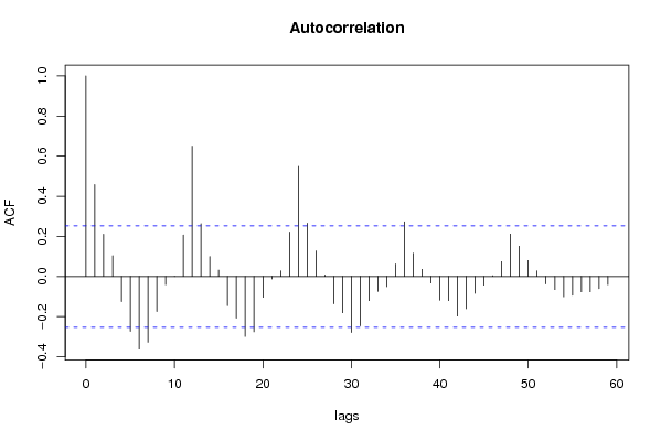
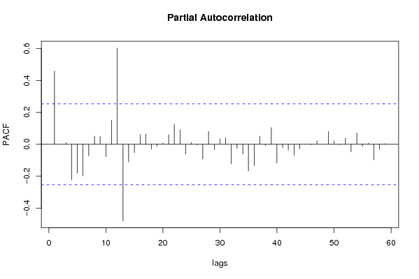
Title produced by software

(Partial) Autocorrelation Function

Date of computation

Thu, 04 Dec 2008 11:21:05 -0700

Cite this page as follows

Statistical Computations at FreeStatistics.org, Office for Research Development and Education, URL https://freestatistics.org/blog/index.php?v=date/2008/Dec/04/t1228414942zd7h79dg73czbt9.htm/, Retrieved Wed, 24 Apr 2024 10:39:03 +0000

Statistical Computations at FreeStatistics.org, Office for Research Development and Education, URL https://freestatistics.org/blog/index.php?pk=28997, Retrieved Wed, 24 Apr 2024 10:39:03 +0000

QR Codes:

Paste this QR Code to cite your computation.

Original text written by user:

IsPrivate?

No (this computation is public)

User-defined keywords

Estimated Impact

268

Family? (F = Feedback message, R = changed R code, M = changed R Module, P = changed Parameters, D = changed Data)

-     [Univariate Data Series] [data set] [2008-12-01 19:54:57] [b98453cac15ba1066b407e146608df68]
F RMP   [(Partial) Autocorrelation Function] [Taak 10 Stap 2 AC...] [2008-12-03 15:12:42] [6fea0e9a9b3b29a63badf2c274e82506]
-    D      [(Partial) Autocorrelation Function] [Taak 10 Stap 2 AC...] [2008-12-04 18:21:05] [e08fee3874f3333d6b7a377a061b860d] [Current]
-   P         [(Partial) Autocorrelation Function] [Taak 10 deel 2 st...] [2008-12-05 13:18:35] [6fea0e9a9b3b29a63badf2c274e82506] 
-   P           [(Partial) Autocorrelation Function] [Taak 10 deel 2 st...] [2008-12-05 13:24:16] [6fea0e9a9b3b29a63badf2c274e82506] 
-   P             [(Partial) Autocorrelation Function] [Taak 10 deel 2 st...] [2008-12-05 13:28:10] [6fea0e9a9b3b29a63badf2c274e82506] 
F             [(Partial) Autocorrelation Function] [stap 2] [2008-12-08 16:33:12] [74be16979710d4c4e7c6647856088456] 
-   P           [(Partial) Autocorrelation Function] [Verbetering ACF s...] [2008-12-15 20:47:34] [bc937651ef42bf891200cf0e0edc7238] 
- RMP             [Spectral Analysis] [Verbetering SA st...] [2008-12-15 20:50:37] [bc937651ef42bf891200cf0e0edc7238] 
- R P         [(Partial) Autocorrelation Function] [Step 2 D=1 en d=1] [2008-12-08 16:44:02] [7458e879e85b911182071700fff19fbd] 
F   P         [(Partial) Autocorrelation Function] [Taak 10 Stap 2 AC...] [2008-12-08 16:54:24] [6fea0e9a9b3b29a63badf2c274e82506] 
-   P           [(Partial) Autocorrelation Function] [Identification an...] [2008-12-08 19:21:03] [79c17183721a40a589db5f9f561947d8] 
F   P         [(Partial) Autocorrelation Function] [Taak 10 deel 2 st...] [2008-12-08 16:56:20] [6fea0e9a9b3b29a63badf2c274e82506] 
-   P           [(Partial) Autocorrelation Function] [Identification an...] [2008-12-08 19:23:00] [79c17183721a40a589db5f9f561947d8] 

Feedback Forum

Post a new message

Dataseries X:

Download CSV

Histogram

Boxplots

Summary of computational transaction
Raw Input	view raw input (R code)
Raw Output	view raw output of R engine
Computing time	1 seconds
R Server	'Gwilym Jenkins' @ 72.249.127.135

\begin{tabular}{lllllllll}
\hline
Summary of computational transaction \tabularnewline
Raw Input & view raw input (R code)  \tabularnewline
Raw Output & view raw output of R engine  \tabularnewline
Computing time & 1 seconds \tabularnewline
R Server & 'Gwilym Jenkins' @ 72.249.127.135 \tabularnewline
\hline
\end{tabular}
%Source: https://freestatistics.org/blog/index.php?pk=28997&T=0

[TABLE]
[ROW][C]Summary of computational transaction[/C][/ROW]
[ROW][C]Raw Input[/C][C]view raw input (R code) [/C][/ROW]
[ROW][C]Raw Output[/C][C]view raw output of R engine [/C][/ROW]
[ROW][C]Computing time[/C][C]1 seconds[/C][/ROW]
[ROW][C]R Server[/C][C]'Gwilym Jenkins' @ 72.249.127.135[/C][/ROW]
[/TABLE]
Source: https://freestatistics.org/blog/index.php?pk=28997&T=0

Globally Unique Identifier (entire table): ba.freestatistics.org/blog/index.php?pk=28997&T=0

As an alternative you can also use a QR Code:

The GUIDs for individual cells are displayed in the table below:

Summary of computational transaction
Raw Input	view raw input (R code)
Raw Output	view raw output of R engine
Computing time	1 seconds
R Server	'Gwilym Jenkins' @ 72.249.127.135

Autocorrelation Function
Time lag k	ACF(k)	T-STAT	P-value
1	0.458592	3.5522	0.000375
2	0.210396	1.6297	0.0542
3	0.103312	0.8003	0.21336
4	-0.125776	-0.9743	0.16692
5	-0.273851	-2.1212	0.019021
6	-0.362472	-2.8077	0.003361
7	-0.328529	-2.5448	0.006763
8	-0.175149	-1.3567	0.08998
9	-0.041032	-0.3178	0.375858
10	-0.000388	-0.003	0.498805
11	0.206423	1.5989	0.057543
12	0.649892	5.034	2e-06
13	0.26275	2.0353	0.023125
14	0.09964	0.7718	0.221628
15	0.031356	0.2429	0.404463
16	-0.146257	-1.1329	0.130882
17	-0.207987	-1.6111	0.056208
18	-0.299245	-2.3179	0.01194
19	-0.276027	-2.1381	0.018296
20	-0.104384	-0.8086	0.210984
21	-0.012813	-0.0992	0.460637
22	0.027626	0.214	0.415639
23	0.221841	1.7184	0.045443
24	0.548841	4.2513	3.8e-05
25	0.265682	2.058	0.021973
26	0.127665	0.9889	0.163345
27	0.007247	0.0561	0.477711
28	-0.136443	-1.0569	0.1474
29	-0.180994	-1.402	0.083037
30	-0.279242	-2.163	0.017268
31	-0.246585	-1.91	0.030456
32	-0.120351	-0.9322	0.177476
33	-0.074887	-0.5801	0.28202
34	-0.05131	-0.3974	0.346225
35	0.062531	0.4844	0.314946
36	0.272905	2.1139	0.019344
37	0.115915	0.8979	0.18642
38	0.03545	0.2746	0.392286
39	-0.032603	-0.2525	0.400743
40	-0.11842	-0.9173	0.181334
41	-0.120507	-0.9334	0.177166
42	-0.197982	-1.5336	0.065197
43	-0.161178	-1.2485	0.108352
44	-0.083937	-0.6502	0.259031
45	-0.043746	-0.3389	0.367951
46	0.003779	0.0293	0.488372
47	0.074241	0.5751	0.283696
48	0.21158	1.6389	0.053235
49	0.15061	1.1666	0.123991
50	0.07973	0.6176	0.269593
51	0.027506	0.2131	0.416001
52	-0.037576	-0.2911	0.386005
53	-0.065907	-0.5105	0.305781
54	-0.10166	-0.7875	0.217058
55	-0.093764	-0.7263	0.235241
56	-0.076517	-0.5927	0.277804
57	-0.076311	-0.5911	0.278335
58	-0.060552	-0.469	0.320373
59	-0.041127	-0.3186	0.375579
60	NA	NA	NA

\begin{tabular}{lllllllll}
\hline
Autocorrelation Function \tabularnewline
Time lag k & ACF(k) & T-STAT & P-value \tabularnewline
1 & 0.458592 & 3.5522 & 0.000375 \tabularnewline
2 & 0.210396 & 1.6297 & 0.0542 \tabularnewline
3 & 0.103312 & 0.8003 & 0.21336 \tabularnewline
4 & -0.125776 & -0.9743 & 0.16692 \tabularnewline
5 & -0.273851 & -2.1212 & 0.019021 \tabularnewline
6 & -0.362472 & -2.8077 & 0.003361 \tabularnewline
7 & -0.328529 & -2.5448 & 0.006763 \tabularnewline
8 & -0.175149 & -1.3567 & 0.08998 \tabularnewline
9 & -0.041032 & -0.3178 & 0.375858 \tabularnewline
10 & -0.000388 & -0.003 & 0.498805 \tabularnewline
11 & 0.206423 & 1.5989 & 0.057543 \tabularnewline
12 & 0.649892 & 5.034 & 2e-06 \tabularnewline
13 & 0.26275 & 2.0353 & 0.023125 \tabularnewline
14 & 0.09964 & 0.7718 & 0.221628 \tabularnewline
15 & 0.031356 & 0.2429 & 0.404463 \tabularnewline
16 & -0.146257 & -1.1329 & 0.130882 \tabularnewline
17 & -0.207987 & -1.6111 & 0.056208 \tabularnewline
18 & -0.299245 & -2.3179 & 0.01194 \tabularnewline
19 & -0.276027 & -2.1381 & 0.018296 \tabularnewline
20 & -0.104384 & -0.8086 & 0.210984 \tabularnewline
21 & -0.012813 & -0.0992 & 0.460637 \tabularnewline
22 & 0.027626 & 0.214 & 0.415639 \tabularnewline
23 & 0.221841 & 1.7184 & 0.045443 \tabularnewline
24 & 0.548841 & 4.2513 & 3.8e-05 \tabularnewline
25 & 0.265682 & 2.058 & 0.021973 \tabularnewline
26 & 0.127665 & 0.9889 & 0.163345 \tabularnewline
27 & 0.007247 & 0.0561 & 0.477711 \tabularnewline
28 & -0.136443 & -1.0569 & 0.1474 \tabularnewline
29 & -0.180994 & -1.402 & 0.083037 \tabularnewline
30 & -0.279242 & -2.163 & 0.017268 \tabularnewline
31 & -0.246585 & -1.91 & 0.030456 \tabularnewline
32 & -0.120351 & -0.9322 & 0.177476 \tabularnewline
33 & -0.074887 & -0.5801 & 0.28202 \tabularnewline
34 & -0.05131 & -0.3974 & 0.346225 \tabularnewline
35 & 0.062531 & 0.4844 & 0.314946 \tabularnewline
36 & 0.272905 & 2.1139 & 0.019344 \tabularnewline
37 & 0.115915 & 0.8979 & 0.18642 \tabularnewline
38 & 0.03545 & 0.2746 & 0.392286 \tabularnewline
39 & -0.032603 & -0.2525 & 0.400743 \tabularnewline
40 & -0.11842 & -0.9173 & 0.181334 \tabularnewline
41 & -0.120507 & -0.9334 & 0.177166 \tabularnewline
42 & -0.197982 & -1.5336 & 0.065197 \tabularnewline
43 & -0.161178 & -1.2485 & 0.108352 \tabularnewline
44 & -0.083937 & -0.6502 & 0.259031 \tabularnewline
45 & -0.043746 & -0.3389 & 0.367951 \tabularnewline
46 & 0.003779 & 0.0293 & 0.488372 \tabularnewline
47 & 0.074241 & 0.5751 & 0.283696 \tabularnewline
48 & 0.21158 & 1.6389 & 0.053235 \tabularnewline
49 & 0.15061 & 1.1666 & 0.123991 \tabularnewline
50 & 0.07973 & 0.6176 & 0.269593 \tabularnewline
51 & 0.027506 & 0.2131 & 0.416001 \tabularnewline
52 & -0.037576 & -0.2911 & 0.386005 \tabularnewline
53 & -0.065907 & -0.5105 & 0.305781 \tabularnewline
54 & -0.10166 & -0.7875 & 0.217058 \tabularnewline
55 & -0.093764 & -0.7263 & 0.235241 \tabularnewline
56 & -0.076517 & -0.5927 & 0.277804 \tabularnewline
57 & -0.076311 & -0.5911 & 0.278335 \tabularnewline
58 & -0.060552 & -0.469 & 0.320373 \tabularnewline
59 & -0.041127 & -0.3186 & 0.375579 \tabularnewline
60 & NA & NA & NA \tabularnewline
\hline
\end{tabular}
%Source: https://freestatistics.org/blog/index.php?pk=28997&T=1

[TABLE]
[ROW][C]Autocorrelation Function[/C][/ROW]
[ROW][C]Time lag k[/C][C]ACF(k)[/C][C]T-STAT[/C][C]P-value[/C][/ROW]
[ROW][C]1[/C][C]0.458592[/C][C]3.5522[/C][C]0.000375[/C][/ROW]
[ROW][C]2[/C][C]0.210396[/C][C]1.6297[/C][C]0.0542[/C][/ROW]
[ROW][C]3[/C][C]0.103312[/C][C]0.8003[/C][C]0.21336[/C][/ROW]
[ROW][C]4[/C][C]-0.125776[/C][C]-0.9743[/C][C]0.16692[/C][/ROW]
[ROW][C]5[/C][C]-0.273851[/C][C]-2.1212[/C][C]0.019021[/C][/ROW]
[ROW][C]6[/C][C]-0.362472[/C][C]-2.8077[/C][C]0.003361[/C][/ROW]
[ROW][C]7[/C][C]-0.328529[/C][C]-2.5448[/C][C]0.006763[/C][/ROW]
[ROW][C]8[/C][C]-0.175149[/C][C]-1.3567[/C][C]0.08998[/C][/ROW]
[ROW][C]9[/C][C]-0.041032[/C][C]-0.3178[/C][C]0.375858[/C][/ROW]
[ROW][C]10[/C][C]-0.000388[/C][C]-0.003[/C][C]0.498805[/C][/ROW]
[ROW][C]11[/C][C]0.206423[/C][C]1.5989[/C][C]0.057543[/C][/ROW]
[ROW][C]12[/C][C]0.649892[/C][C]5.034[/C][C]2e-06[/C][/ROW]
[ROW][C]13[/C][C]0.26275[/C][C]2.0353[/C][C]0.023125[/C][/ROW]
[ROW][C]14[/C][C]0.09964[/C][C]0.7718[/C][C]0.221628[/C][/ROW]
[ROW][C]15[/C][C]0.031356[/C][C]0.2429[/C][C]0.404463[/C][/ROW]
[ROW][C]16[/C][C]-0.146257[/C][C]-1.1329[/C][C]0.130882[/C][/ROW]
[ROW][C]17[/C][C]-0.207987[/C][C]-1.6111[/C][C]0.056208[/C][/ROW]
[ROW][C]18[/C][C]-0.299245[/C][C]-2.3179[/C][C]0.01194[/C][/ROW]
[ROW][C]19[/C][C]-0.276027[/C][C]-2.1381[/C][C]0.018296[/C][/ROW]
[ROW][C]20[/C][C]-0.104384[/C][C]-0.8086[/C][C]0.210984[/C][/ROW]
[ROW][C]21[/C][C]-0.012813[/C][C]-0.0992[/C][C]0.460637[/C][/ROW]
[ROW][C]22[/C][C]0.027626[/C][C]0.214[/C][C]0.415639[/C][/ROW]
[ROW][C]23[/C][C]0.221841[/C][C]1.7184[/C][C]0.045443[/C][/ROW]
[ROW][C]24[/C][C]0.548841[/C][C]4.2513[/C][C]3.8e-05[/C][/ROW]
[ROW][C]25[/C][C]0.265682[/C][C]2.058[/C][C]0.021973[/C][/ROW]
[ROW][C]26[/C][C]0.127665[/C][C]0.9889[/C][C]0.163345[/C][/ROW]
[ROW][C]27[/C][C]0.007247[/C][C]0.0561[/C][C]0.477711[/C][/ROW]
[ROW][C]28[/C][C]-0.136443[/C][C]-1.0569[/C][C]0.1474[/C][/ROW]
[ROW][C]29[/C][C]-0.180994[/C][C]-1.402[/C][C]0.083037[/C][/ROW]
[ROW][C]30[/C][C]-0.279242[/C][C]-2.163[/C][C]0.017268[/C][/ROW]
[ROW][C]31[/C][C]-0.246585[/C][C]-1.91[/C][C]0.030456[/C][/ROW]
[ROW][C]32[/C][C]-0.120351[/C][C]-0.9322[/C][C]0.177476[/C][/ROW]
[ROW][C]33[/C][C]-0.074887[/C][C]-0.5801[/C][C]0.28202[/C][/ROW]
[ROW][C]34[/C][C]-0.05131[/C][C]-0.3974[/C][C]0.346225[/C][/ROW]
[ROW][C]35[/C][C]0.062531[/C][C]0.4844[/C][C]0.314946[/C][/ROW]
[ROW][C]36[/C][C]0.272905[/C][C]2.1139[/C][C]0.019344[/C][/ROW]
[ROW][C]37[/C][C]0.115915[/C][C]0.8979[/C][C]0.18642[/C][/ROW]
[ROW][C]38[/C][C]0.03545[/C][C]0.2746[/C][C]0.392286[/C][/ROW]
[ROW][C]39[/C][C]-0.032603[/C][C]-0.2525[/C][C]0.400743[/C][/ROW]
[ROW][C]40[/C][C]-0.11842[/C][C]-0.9173[/C][C]0.181334[/C][/ROW]
[ROW][C]41[/C][C]-0.120507[/C][C]-0.9334[/C][C]0.177166[/C][/ROW]
[ROW][C]42[/C][C]-0.197982[/C][C]-1.5336[/C][C]0.065197[/C][/ROW]
[ROW][C]43[/C][C]-0.161178[/C][C]-1.2485[/C][C]0.108352[/C][/ROW]
[ROW][C]44[/C][C]-0.083937[/C][C]-0.6502[/C][C]0.259031[/C][/ROW]
[ROW][C]45[/C][C]-0.043746[/C][C]-0.3389[/C][C]0.367951[/C][/ROW]
[ROW][C]46[/C][C]0.003779[/C][C]0.0293[/C][C]0.488372[/C][/ROW]
[ROW][C]47[/C][C]0.074241[/C][C]0.5751[/C][C]0.283696[/C][/ROW]
[ROW][C]48[/C][C]0.21158[/C][C]1.6389[/C][C]0.053235[/C][/ROW]
[ROW][C]49[/C][C]0.15061[/C][C]1.1666[/C][C]0.123991[/C][/ROW]
[ROW][C]50[/C][C]0.07973[/C][C]0.6176[/C][C]0.269593[/C][/ROW]
[ROW][C]51[/C][C]0.027506[/C][C]0.2131[/C][C]0.416001[/C][/ROW]
[ROW][C]52[/C][C]-0.037576[/C][C]-0.2911[/C][C]0.386005[/C][/ROW]
[ROW][C]53[/C][C]-0.065907[/C][C]-0.5105[/C][C]0.305781[/C][/ROW]
[ROW][C]54[/C][C]-0.10166[/C][C]-0.7875[/C][C]0.217058[/C][/ROW]
[ROW][C]55[/C][C]-0.093764[/C][C]-0.7263[/C][C]0.235241[/C][/ROW]
[ROW][C]56[/C][C]-0.076517[/C][C]-0.5927[/C][C]0.277804[/C][/ROW]
[ROW][C]57[/C][C]-0.076311[/C][C]-0.5911[/C][C]0.278335[/C][/ROW]
[ROW][C]58[/C][C]-0.060552[/C][C]-0.469[/C][C]0.320373[/C][/ROW]
[ROW][C]59[/C][C]-0.041127[/C][C]-0.3186[/C][C]0.375579[/C][/ROW]
[ROW][C]60[/C][C]NA[/C][C]NA[/C][C]NA[/C][/ROW]
[/TABLE]
Source: https://freestatistics.org/blog/index.php?pk=28997&T=1

Globally Unique Identifier (entire table): ba.freestatistics.org/blog/index.php?pk=28997&T=1

As an alternative you can also use a QR Code:

The GUIDs for individual cells are displayed in the table below:

Autocorrelation Function
Time lag k	ACF(k)	T-STAT	P-value
1	0.458592	3.5522	0.000375
2	0.210396	1.6297	0.0542
3	0.103312	0.8003	0.21336
4	-0.125776	-0.9743	0.16692
5	-0.273851	-2.1212	0.019021
6	-0.362472	-2.8077	0.003361
7	-0.328529	-2.5448	0.006763
8	-0.175149	-1.3567	0.08998
9	-0.041032	-0.3178	0.375858
10	-0.000388	-0.003	0.498805
11	0.206423	1.5989	0.057543
12	0.649892	5.034	2e-06
13	0.26275	2.0353	0.023125
14	0.09964	0.7718	0.221628
15	0.031356	0.2429	0.404463
16	-0.146257	-1.1329	0.130882
17	-0.207987	-1.6111	0.056208
18	-0.299245	-2.3179	0.01194
19	-0.276027	-2.1381	0.018296
20	-0.104384	-0.8086	0.210984
21	-0.012813	-0.0992	0.460637
22	0.027626	0.214	0.415639
23	0.221841	1.7184	0.045443
24	0.548841	4.2513	3.8e-05
25	0.265682	2.058	0.021973
26	0.127665	0.9889	0.163345
27	0.007247	0.0561	0.477711
28	-0.136443	-1.0569	0.1474
29	-0.180994	-1.402	0.083037
30	-0.279242	-2.163	0.017268
31	-0.246585	-1.91	0.030456
32	-0.120351	-0.9322	0.177476
33	-0.074887	-0.5801	0.28202
34	-0.05131	-0.3974	0.346225
35	0.062531	0.4844	0.314946
36	0.272905	2.1139	0.019344
37	0.115915	0.8979	0.18642
38	0.03545	0.2746	0.392286
39	-0.032603	-0.2525	0.400743
40	-0.11842	-0.9173	0.181334
41	-0.120507	-0.9334	0.177166
42	-0.197982	-1.5336	0.065197
43	-0.161178	-1.2485	0.108352
44	-0.083937	-0.6502	0.259031
45	-0.043746	-0.3389	0.367951
46	0.003779	0.0293	0.488372
47	0.074241	0.5751	0.283696
48	0.21158	1.6389	0.053235
49	0.15061	1.1666	0.123991
50	0.07973	0.6176	0.269593
51	0.027506	0.2131	0.416001
52	-0.037576	-0.2911	0.386005
53	-0.065907	-0.5105	0.305781
54	-0.10166	-0.7875	0.217058
55	-0.093764	-0.7263	0.235241
56	-0.076517	-0.5927	0.277804
57	-0.076311	-0.5911	0.278335
58	-0.060552	-0.469	0.320373
59	-0.041127	-0.3186	0.375579
60	NA	NA	NA

Partial Autocorrelation Function
Time lag k	PACF(k)	T-STAT	P-value
1	0.458592	3.5522	0.000375
2	0.000113	9e-04	0.499652
3	0.008593	0.0666	0.473576
4	-0.223248	-1.7293	0.044452
5	-0.181824	-1.4084	0.082087
6	-0.198739	-1.5394	0.064479
7	-0.072114	-0.5586	0.289258
8	0.051943	0.4024	0.344427
9	0.048834	0.3783	0.353284
10	-0.076874	-0.5955	0.276887
11	0.149476	1.1578	0.12576
12	0.602391	4.6661	9e-06
13	-0.479722	-3.7159	0.000223
14	-0.111196	-0.8613	0.196245
15	-0.051653	-0.4001	0.345252
16	0.060066	0.4653	0.321713
17	0.063751	0.4938	0.311621
18	-0.030578	-0.2369	0.406787
19	-0.014323	-0.1109	0.456014
20	0.007428	0.0575	0.477155
21	0.060195	0.4663	0.321357
22	0.124322	0.963	0.169708
23	0.091495	0.7087	0.240622
24	-0.061442	-0.4759	0.317926
25	0.010708	0.0829	0.467086
26	-0.003474	-0.0269	0.489312
27	-0.092755	-0.7185	0.237627
28	0.079741	0.6177	0.269565
29	-0.035073	-0.2717	0.393404
30	0.033133	0.2566	0.399164
31	0.040653	0.3149	0.376966
32	-0.123179	-0.9541	0.17192
33	-0.025995	-0.2014	0.42055
34	-0.061093	-0.4732	0.318885
35	-0.167642	-1.2985	0.099534
36	-0.133358	-1.033	0.152878
37	0.050886	0.3942	0.34743
38	-0.007552	-0.0585	0.476774
39	0.104273	0.8077	0.211229
40	-0.117192	-0.9078	0.183816
41	-0.021422	-0.1659	0.434384
42	-0.036298	-0.2812	0.389776
43	-0.069975	-0.542	0.294904
44	-0.029102	-0.2254	0.411208
45	0.000833	0.0065	0.497437
46	-0.002199	-0.017	0.493234
47	0.020825	0.1613	0.436194
48	0.000448	0.0035	0.49862
49	0.079421	0.6152	0.270377
50	0.021563	0.167	0.433956
51	-0.002438	-0.0189	0.492499
52	0.038893	0.3013	0.382128
53	-0.047996	-0.3718	0.355685
54	0.071221	0.5517	0.29161
55	-0.012994	-0.1007	0.460082
56	0.006887	0.0533	0.478815
57	-0.097563	-0.7557	0.226387
58	-0.032737	-0.2536	0.400342
59	0.00429	0.0332	0.486802
60	NA	NA	NA

\begin{tabular}{lllllllll}
\hline
Partial Autocorrelation Function \tabularnewline
Time lag k & PACF(k) & T-STAT & P-value \tabularnewline
1 & 0.458592 & 3.5522 & 0.000375 \tabularnewline
2 & 0.000113 & 9e-04 & 0.499652 \tabularnewline
3 & 0.008593 & 0.0666 & 0.473576 \tabularnewline
4 & -0.223248 & -1.7293 & 0.044452 \tabularnewline
5 & -0.181824 & -1.4084 & 0.082087 \tabularnewline
6 & -0.198739 & -1.5394 & 0.064479 \tabularnewline
7 & -0.072114 & -0.5586 & 0.289258 \tabularnewline
8 & 0.051943 & 0.4024 & 0.344427 \tabularnewline
9 & 0.048834 & 0.3783 & 0.353284 \tabularnewline
10 & -0.076874 & -0.5955 & 0.276887 \tabularnewline
11 & 0.149476 & 1.1578 & 0.12576 \tabularnewline
12 & 0.602391 & 4.6661 & 9e-06 \tabularnewline
13 & -0.479722 & -3.7159 & 0.000223 \tabularnewline
14 & -0.111196 & -0.8613 & 0.196245 \tabularnewline
15 & -0.051653 & -0.4001 & 0.345252 \tabularnewline
16 & 0.060066 & 0.4653 & 0.321713 \tabularnewline
17 & 0.063751 & 0.4938 & 0.311621 \tabularnewline
18 & -0.030578 & -0.2369 & 0.406787 \tabularnewline
19 & -0.014323 & -0.1109 & 0.456014 \tabularnewline
20 & 0.007428 & 0.0575 & 0.477155 \tabularnewline
21 & 0.060195 & 0.4663 & 0.321357 \tabularnewline
22 & 0.124322 & 0.963 & 0.169708 \tabularnewline
23 & 0.091495 & 0.7087 & 0.240622 \tabularnewline
24 & -0.061442 & -0.4759 & 0.317926 \tabularnewline
25 & 0.010708 & 0.0829 & 0.467086 \tabularnewline
26 & -0.003474 & -0.0269 & 0.489312 \tabularnewline
27 & -0.092755 & -0.7185 & 0.237627 \tabularnewline
28 & 0.079741 & 0.6177 & 0.269565 \tabularnewline
29 & -0.035073 & -0.2717 & 0.393404 \tabularnewline
30 & 0.033133 & 0.2566 & 0.399164 \tabularnewline
31 & 0.040653 & 0.3149 & 0.376966 \tabularnewline
32 & -0.123179 & -0.9541 & 0.17192 \tabularnewline
33 & -0.025995 & -0.2014 & 0.42055 \tabularnewline
34 & -0.061093 & -0.4732 & 0.318885 \tabularnewline
35 & -0.167642 & -1.2985 & 0.099534 \tabularnewline
36 & -0.133358 & -1.033 & 0.152878 \tabularnewline
37 & 0.050886 & 0.3942 & 0.34743 \tabularnewline
38 & -0.007552 & -0.0585 & 0.476774 \tabularnewline
39 & 0.104273 & 0.8077 & 0.211229 \tabularnewline
40 & -0.117192 & -0.9078 & 0.183816 \tabularnewline
41 & -0.021422 & -0.1659 & 0.434384 \tabularnewline
42 & -0.036298 & -0.2812 & 0.389776 \tabularnewline
43 & -0.069975 & -0.542 & 0.294904 \tabularnewline
44 & -0.029102 & -0.2254 & 0.411208 \tabularnewline
45 & 0.000833 & 0.0065 & 0.497437 \tabularnewline
46 & -0.002199 & -0.017 & 0.493234 \tabularnewline
47 & 0.020825 & 0.1613 & 0.436194 \tabularnewline
48 & 0.000448 & 0.0035 & 0.49862 \tabularnewline
49 & 0.079421 & 0.6152 & 0.270377 \tabularnewline
50 & 0.021563 & 0.167 & 0.433956 \tabularnewline
51 & -0.002438 & -0.0189 & 0.492499 \tabularnewline
52 & 0.038893 & 0.3013 & 0.382128 \tabularnewline
53 & -0.047996 & -0.3718 & 0.355685 \tabularnewline
54 & 0.071221 & 0.5517 & 0.29161 \tabularnewline
55 & -0.012994 & -0.1007 & 0.460082 \tabularnewline
56 & 0.006887 & 0.0533 & 0.478815 \tabularnewline
57 & -0.097563 & -0.7557 & 0.226387 \tabularnewline
58 & -0.032737 & -0.2536 & 0.400342 \tabularnewline
59 & 0.00429 & 0.0332 & 0.486802 \tabularnewline
60 & NA & NA & NA \tabularnewline
\hline
\end{tabular}
%Source: https://freestatistics.org/blog/index.php?pk=28997&T=2

[TABLE]
[ROW][C]Partial Autocorrelation Function[/C][/ROW]
[ROW][C]Time lag k[/C][C]PACF(k)[/C][C]T-STAT[/C][C]P-value[/C][/ROW]
[ROW][C]1[/C][C]0.458592[/C][C]3.5522[/C][C]0.000375[/C][/ROW]
[ROW][C]2[/C][C]0.000113[/C][C]9e-04[/C][C]0.499652[/C][/ROW]
[ROW][C]3[/C][C]0.008593[/C][C]0.0666[/C][C]0.473576[/C][/ROW]
[ROW][C]4[/C][C]-0.223248[/C][C]-1.7293[/C][C]0.044452[/C][/ROW]
[ROW][C]5[/C][C]-0.181824[/C][C]-1.4084[/C][C]0.082087[/C][/ROW]
[ROW][C]6[/C][C]-0.198739[/C][C]-1.5394[/C][C]0.064479[/C][/ROW]
[ROW][C]7[/C][C]-0.072114[/C][C]-0.5586[/C][C]0.289258[/C][/ROW]
[ROW][C]8[/C][C]0.051943[/C][C]0.4024[/C][C]0.344427[/C][/ROW]
[ROW][C]9[/C][C]0.048834[/C][C]0.3783[/C][C]0.353284[/C][/ROW]
[ROW][C]10[/C][C]-0.076874[/C][C]-0.5955[/C][C]0.276887[/C][/ROW]
[ROW][C]11[/C][C]0.149476[/C][C]1.1578[/C][C]0.12576[/C][/ROW]
[ROW][C]12[/C][C]0.602391[/C][C]4.6661[/C][C]9e-06[/C][/ROW]
[ROW][C]13[/C][C]-0.479722[/C][C]-3.7159[/C][C]0.000223[/C][/ROW]
[ROW][C]14[/C][C]-0.111196[/C][C]-0.8613[/C][C]0.196245[/C][/ROW]
[ROW][C]15[/C][C]-0.051653[/C][C]-0.4001[/C][C]0.345252[/C][/ROW]
[ROW][C]16[/C][C]0.060066[/C][C]0.4653[/C][C]0.321713[/C][/ROW]
[ROW][C]17[/C][C]0.063751[/C][C]0.4938[/C][C]0.311621[/C][/ROW]
[ROW][C]18[/C][C]-0.030578[/C][C]-0.2369[/C][C]0.406787[/C][/ROW]
[ROW][C]19[/C][C]-0.014323[/C][C]-0.1109[/C][C]0.456014[/C][/ROW]
[ROW][C]20[/C][C]0.007428[/C][C]0.0575[/C][C]0.477155[/C][/ROW]
[ROW][C]21[/C][C]0.060195[/C][C]0.4663[/C][C]0.321357[/C][/ROW]
[ROW][C]22[/C][C]0.124322[/C][C]0.963[/C][C]0.169708[/C][/ROW]
[ROW][C]23[/C][C]0.091495[/C][C]0.7087[/C][C]0.240622[/C][/ROW]
[ROW][C]24[/C][C]-0.061442[/C][C]-0.4759[/C][C]0.317926[/C][/ROW]
[ROW][C]25[/C][C]0.010708[/C][C]0.0829[/C][C]0.467086[/C][/ROW]
[ROW][C]26[/C][C]-0.003474[/C][C]-0.0269[/C][C]0.489312[/C][/ROW]
[ROW][C]27[/C][C]-0.092755[/C][C]-0.7185[/C][C]0.237627[/C][/ROW]
[ROW][C]28[/C][C]0.079741[/C][C]0.6177[/C][C]0.269565[/C][/ROW]
[ROW][C]29[/C][C]-0.035073[/C][C]-0.2717[/C][C]0.393404[/C][/ROW]
[ROW][C]30[/C][C]0.033133[/C][C]0.2566[/C][C]0.399164[/C][/ROW]
[ROW][C]31[/C][C]0.040653[/C][C]0.3149[/C][C]0.376966[/C][/ROW]
[ROW][C]32[/C][C]-0.123179[/C][C]-0.9541[/C][C]0.17192[/C][/ROW]
[ROW][C]33[/C][C]-0.025995[/C][C]-0.2014[/C][C]0.42055[/C][/ROW]
[ROW][C]34[/C][C]-0.061093[/C][C]-0.4732[/C][C]0.318885[/C][/ROW]
[ROW][C]35[/C][C]-0.167642[/C][C]-1.2985[/C][C]0.099534[/C][/ROW]
[ROW][C]36[/C][C]-0.133358[/C][C]-1.033[/C][C]0.152878[/C][/ROW]
[ROW][C]37[/C][C]0.050886[/C][C]0.3942[/C][C]0.34743[/C][/ROW]
[ROW][C]38[/C][C]-0.007552[/C][C]-0.0585[/C][C]0.476774[/C][/ROW]
[ROW][C]39[/C][C]0.104273[/C][C]0.8077[/C][C]0.211229[/C][/ROW]
[ROW][C]40[/C][C]-0.117192[/C][C]-0.9078[/C][C]0.183816[/C][/ROW]
[ROW][C]41[/C][C]-0.021422[/C][C]-0.1659[/C][C]0.434384[/C][/ROW]
[ROW][C]42[/C][C]-0.036298[/C][C]-0.2812[/C][C]0.389776[/C][/ROW]
[ROW][C]43[/C][C]-0.069975[/C][C]-0.542[/C][C]0.294904[/C][/ROW]
[ROW][C]44[/C][C]-0.029102[/C][C]-0.2254[/C][C]0.411208[/C][/ROW]
[ROW][C]45[/C][C]0.000833[/C][C]0.0065[/C][C]0.497437[/C][/ROW]
[ROW][C]46[/C][C]-0.002199[/C][C]-0.017[/C][C]0.493234[/C][/ROW]
[ROW][C]47[/C][C]0.020825[/C][C]0.1613[/C][C]0.436194[/C][/ROW]
[ROW][C]48[/C][C]0.000448[/C][C]0.0035[/C][C]0.49862[/C][/ROW]
[ROW][C]49[/C][C]0.079421[/C][C]0.6152[/C][C]0.270377[/C][/ROW]
[ROW][C]50[/C][C]0.021563[/C][C]0.167[/C][C]0.433956[/C][/ROW]
[ROW][C]51[/C][C]-0.002438[/C][C]-0.0189[/C][C]0.492499[/C][/ROW]
[ROW][C]52[/C][C]0.038893[/C][C]0.3013[/C][C]0.382128[/C][/ROW]
[ROW][C]53[/C][C]-0.047996[/C][C]-0.3718[/C][C]0.355685[/C][/ROW]
[ROW][C]54[/C][C]0.071221[/C][C]0.5517[/C][C]0.29161[/C][/ROW]
[ROW][C]55[/C][C]-0.012994[/C][C]-0.1007[/C][C]0.460082[/C][/ROW]
[ROW][C]56[/C][C]0.006887[/C][C]0.0533[/C][C]0.478815[/C][/ROW]
[ROW][C]57[/C][C]-0.097563[/C][C]-0.7557[/C][C]0.226387[/C][/ROW]
[ROW][C]58[/C][C]-0.032737[/C][C]-0.2536[/C][C]0.400342[/C][/ROW]
[ROW][C]59[/C][C]0.00429[/C][C]0.0332[/C][C]0.486802[/C][/ROW]
[ROW][C]60[/C][C]NA[/C][C]NA[/C][C]NA[/C][/ROW]
[/TABLE]
Source: https://freestatistics.org/blog/index.php?pk=28997&T=2

Globally Unique Identifier (entire table): ba.freestatistics.org/blog/index.php?pk=28997&T=2

As an alternative you can also use a QR Code:

The GUIDs for individual cells are displayed in the table below:

Partial Autocorrelation Function
Time lag k	PACF(k)	T-STAT	P-value
1	0.458592	3.5522	0.000375
2	0.000113	9e-04	0.499652
3	0.008593	0.0666	0.473576
4	-0.223248	-1.7293	0.044452
5	-0.181824	-1.4084	0.082087
6	-0.198739	-1.5394	0.064479
7	-0.072114	-0.5586	0.289258
8	0.051943	0.4024	0.344427
9	0.048834	0.3783	0.353284
10	-0.076874	-0.5955	0.276887
11	0.149476	1.1578	0.12576
12	0.602391	4.6661	9e-06
13	-0.479722	-3.7159	0.000223
14	-0.111196	-0.8613	0.196245
15	-0.051653	-0.4001	0.345252
16	0.060066	0.4653	0.321713
17	0.063751	0.4938	0.311621
18	-0.030578	-0.2369	0.406787
19	-0.014323	-0.1109	0.456014
20	0.007428	0.0575	0.477155
21	0.060195	0.4663	0.321357
22	0.124322	0.963	0.169708
23	0.091495	0.7087	0.240622
24	-0.061442	-0.4759	0.317926
25	0.010708	0.0829	0.467086
26	-0.003474	-0.0269	0.489312
27	-0.092755	-0.7185	0.237627
28	0.079741	0.6177	0.269565
29	-0.035073	-0.2717	0.393404
30	0.033133	0.2566	0.399164
31	0.040653	0.3149	0.376966
32	-0.123179	-0.9541	0.17192
33	-0.025995	-0.2014	0.42055
34	-0.061093	-0.4732	0.318885
35	-0.167642	-1.2985	0.099534
36	-0.133358	-1.033	0.152878
37	0.050886	0.3942	0.34743
38	-0.007552	-0.0585	0.476774
39	0.104273	0.8077	0.211229
40	-0.117192	-0.9078	0.183816
41	-0.021422	-0.1659	0.434384
42	-0.036298	-0.2812	0.389776
43	-0.069975	-0.542	0.294904
44	-0.029102	-0.2254	0.411208
45	0.000833	0.0065	0.497437
46	-0.002199	-0.017	0.493234
47	0.020825	0.1613	0.436194
48	0.000448	0.0035	0.49862
49	0.079421	0.6152	0.270377
50	0.021563	0.167	0.433956
51	-0.002438	-0.0189	0.492499
52	0.038893	0.3013	0.382128
53	-0.047996	-0.3718	0.355685
54	0.071221	0.5517	0.29161
55	-0.012994	-0.1007	0.460082
56	0.006887	0.0533	0.478815
57	-0.097563	-0.7557	0.226387
58	-0.032737	-0.2536	0.400342
59	0.00429	0.0332	0.486802
60	NA	NA	NA

Figure 1

PNG link

Postscript link

PDF link

Figure 2

PNG link

Postscript link

PDF link

Parameters (Session):

par1 = 60 ; par2 = 1 ; par3 = 0 ; par4 = 0 ; par5 = 12 ;

Parameters (R input):

par1 = 60 ; par2 = 1 ; par3 = 0 ; par4 = 0 ; par5 = 12 ;

R code (references can be found in the software module):

if (par1 == 'Default') {
par1 = 10*log10(length(x))
} else {
par1 <- as.numeric(par1)
}
par2 <- as.numeric(par2)
par3 <- as.numeric(par3)
par4 <- as.numeric(par4)
par5 <- as.numeric(par5)
if (par2 == 0) {
x <- log(x)
} else {
x <- (x ^ par2 - 1) / par2
}
if (par3 > 0) x <- diff(x,lag=1,difference=par3)
if (par4 > 0) x <- diff(x,lag=par5,difference=par4)
bitmap(file='pic1.png')
racf <- acf(x,par1,main='Autocorrelation',xlab='lags',ylab='ACF')
dev.off()
bitmap(file='pic2.png')
rpacf <- pacf(x,par1,main='Partial Autocorrelation',xlab='lags',ylab='PACF')
dev.off()
(myacf <- c(racf$acf))
(mypacf <- c(rpacf$acf))
lengthx <- length(x)
sqrtn <- sqrt(lengthx)
load(file='createtable')
a<-table.start()
a<-table.row.start(a)
a<-table.element(a,'Autocorrelation Function',4,TRUE)
a<-table.row.end(a)
a<-table.row.start(a)
a<-table.element(a,'Time lag k',header=TRUE)
a<-table.element(a,hyperlink('basics.htm','ACF(k)','click here for more information about the Autocorrelation Function'),header=TRUE)
a<-table.element(a,'T-STAT',header=TRUE)
a<-table.element(a,'P-value',header=TRUE)
a<-table.row.end(a)
for (i in 2:(par1+1)) {
a<-table.row.start(a)
a<-table.element(a,i-1,header=TRUE)
a<-table.element(a,round(myacf[i],6))
mytstat <- myacf[i]*sqrtn
a<-table.element(a,round(mytstat,4))
a<-table.element(a,round(1-pt(abs(mytstat),lengthx),6))
a<-table.row.end(a)
}
a<-table.end(a)
table.save(a,file='mytable.tab')
a<-table.start()
a<-table.row.start(a)
a<-table.element(a,'Partial Autocorrelation Function',4,TRUE)
a<-table.row.end(a)
a<-table.row.start(a)
a<-table.element(a,'Time lag k',header=TRUE)
a<-table.element(a,hyperlink('basics.htm','PACF(k)','click here for more information about the Partial Autocorrelation Function'),header=TRUE)
a<-table.element(a,'T-STAT',header=TRUE)
a<-table.element(a,'P-value',header=TRUE)
a<-table.row.end(a)
for (i in 1:par1) {
a<-table.row.start(a)
a<-table.element(a,i,header=TRUE)
a<-table.element(a,round(mypacf[i],6))
mytstat <- mypacf[i]*sqrtn
a<-table.element(a,round(mytstat,4))
a<-table.element(a,round(1-pt(abs(mytstat),lengthx),6))
a<-table.row.end(a)
}
a<-table.end(a)
table.save(a,file='mytable1.tab')

Free Statistics

Description of Statistical Computation

Tree of Dependent Computations

Dataset

Tables (Output of Computation)

Figures (Output of Computation)

Input Parameters & R Code