*The author of this computation has been verified*

R Software Module: /rwasp_multipleregression.wasp (opens new window with default values)

Title produced by software: Multiple Regression

Date of computation: Thu, 03 Feb 2011 11:05:16 +0000

Cite this page as follows:

Statistical Computations at FreeStatistics.org, Office for Research Development and Education, URL http://www.freestatistics.org/blog/date/2011/Feb/03/t12967327677r04z1co01m7o8n.htm/, Retrieved Thu, 03 Feb 2011 12:32:47 +0100

BibTeX entries for LaTeX users:

@Manual{KEY, author = {{YOUR NAME}}, publisher = {Office for Research Development and Education}, title = {Statistical Computations at FreeStatistics.org, URL http://www.freestatistics.org/blog/date/2011/Feb/03/t12967327677r04z1co01m7o8n.htm/}, year = {2011}, } @Manual{R, title = {R: A Language and Environment for Statistical Computing}, author = {{R Development Core Team}}, organization = {R Foundation for Statistical Computing}, address = {Vienna, Austria}, year = {2011}, note = {{ISBN} 3-900051-07-0}, url = {http://www.R-project.org}, }

Original text written by user:

IsPrivate?

No (this computation is public)

User-defined keywords:

Dataseries X:

» Textbox « » Textfile « » CSV «

5393 552486 3.90 3.0 628232 5147 516610 3.90 2.2 612117 4846 487587 3.88 2.3 595404 3995 403620 3.89 2.8 597141 4491 459427 3.89 2.8 593408 4676 473058 3.93 2.8 590072 5461 583054 3.94 2.2 579799 4758 509448 3.97 2.6 574205 5302 551582 4.00 2.8 572775 5066 524752 4.04 2.5 572942 3491 370725 4.18 2.4 619567 4944 531443 4.32 2.3 625809 5148 537833 4.37 1.9 619916 5351 551410 4.40 1.7 587625 5178 520983 4.38 2.0 565742 4025 395542 4.36 2.1 557274 4449 442878 4.36 1.7 560576 4594 454919 4.40 1.8 548854 4603 488905 4.41 1.8 531673 4911 496085 4.43 1.8 525919 5236 540146 4.42 1.3 511038 4652 496529 4.46 1.3 498662 3479 372656 4.61 1.3 555362 4556 486704 4.78 1.2 564591 4815 495334 4.88 1.4 541657 4949 504697 4.95 2.2 527070 4499 464856 4.95 2.9 509846 3865 388472 4.93 3.1 514258 3657 377508 4.93 3.5 516922 4814 468895 4.91 3.6 507561 4614 471295 4.88 4.4 492622 4539 482956 4.83 4.1 490243 4492 483404 4.83 5.1 469357 4779 495548 4.85 5.8 477580 3193 333806 4.99 5.9 528379 3894 4116 etc...

Output produced by software:

Enter (or paste) a matrix (table) containing all data (time) series. Every column represents a different variable and must be delimited by a space or Tab. Every row represents a period in time (or category) and must be delimited by hard returns. The easiest way to enter data is to copy and paste a block of spreadsheet cells. Please, do not use commas or spaces to seperate groups of digits! Summary of computational transaction Raw Input view raw input (R code) Raw Output view raw output of R engine Computing time 5 seconds R Server 'Sir Ronald Aylmer Fisher' @ 193.190.124.24 Multiple Linear Regression - Estimated Regression Equation Nieuwe_woningen[t] = + 844.662452502211 + 0.00979992211956494Bewoonbare_opp[t] -59.3550515481143Rentevoet[t] -6.8793584211157Inflatie[t] -0.00111650716825730Werkloosheid[t] + 17.0236839023143M1[t] + 89.6819626476742M2[t] + 79.962177561074M3[t] + 186.938946390054M4[t] + 173.949222694486M5[t] + 184.728747211172M6[t] -16.1847742968401M7[t] -32.3202345478152M8[t] -47.2131196851659M9[t] -24.4999930800091M10[t] + 55.7297902008376M11[t] -3.74058747559312t + e[t] Multiple Linear Regression - Ordinary Least Squares Variable Parameter S.D. T-STAT H0: parameter = 0 2-tail p-value 1-tail p-value (Intercept) 844.662452502211 1439.618344 0.5867 0.560455 0.280228 Bewoonbare_opp 0.00979992211956494 0.000601 16.2962 0 0 Rentevoet -59.3550515481143 117.302948 -0.506 0.615442 0.307721 Inflatie -6.8793584211157 10.986697 -0.6262 0.534524 0.267262 Werkloosheid -0.00111650716825730 0.001364 -0.8187 0.417471 0.208735 M1 17.0236839023143 70.391854 0.2418 0.810053 0.405026 M2 89.6819626476742 76.160693 1.1775 0.245458 0.122729 M3 79.962177561074 91.646186 0.8725 0.387777 0.193888 M4 186.938946390054 116.864317 1.5996 0.117005 0.058502 M5 173.949222694486 104.750321 1.6606 0.104068 0.052034 M6 184.728747211172 102.304092 1.8057 0.077972 0.038986 M7 -16.1847742968401 105.295035 -0.1537 0.878558 0.439279 M8 -32.3202345478152 111.930805 -0.2888 0.774159 0.387079 M9 -47.2131196851659 125.487848 -0.3762 0.708591 0.354296 M10 -24.4999930800091 123.11905 -0.199 0.843205 0.421603 M11 55.7297902008376 108.074598 0.5157 0.608733 0.304366 t -3.74058747559312 1.778528 -2.1032 0.041338 0.020669 Multiple Linear Regression - Regression Statistics Multiple R 0.991425201597058 R-squared 0.982923930361768 Adjusted R-squared 0.97657004398475 F-TEST (value) 154.69649157045 F-TEST (DF numerator) 16 F-TEST (DF denominator) 43 p-value 0 Multiple Linear Regression - Residual Statistics Residual Standard Deviation 109.145148933887 Sum Squared Residuals 512244.532039412 Multiple Linear Regression - Actuals, Interpolation, and Residuals Time or Index Actuals Interpolation Forecast Residuals Prediction Error 1 5393 5318.71701344928 74.2829865507232 2 5147 5059.54869851089 87.4513014891109 3 4846 4780.8245357645 65.1754642355025 4 3995 4055.21805382707 -60.2180538270727 5 4491 4589.55991764158 -98.5599176415771 6 4676 4731.53205894584 -55.5320589458413 7 5461 5619.8341261026 -158.834126102597 8 4758 4880.33835702767 -122.338357027674 9 5302 5273.05488502042 28.9451149795796 10 5066 5028.59866244937 37.4013375506321 11 3491 3535.95633584977 -44.9563358497706 12 4944 5036.91883226669 -92.9188322666921 13 5148 5119.18699857101 28.8130014289860 14 5351 5356.80658556609 -5.80658556609038 15 5178 5068.7198025395 109.280197460503 16 4025 3952.59770118219 72.4022988178093 17 4449 4398.82154016162 50.1784598383832 18 4594 4533.88689856667 60.1131014333332 19 4603 4680.88210188094 -77.8821018809437 20 4911 4736.60677618804 174.393223811958 21 5236 5170.41564498212 65.5843550178749 22 4652 4773.38867167505 -121.388671675052 23 3479 3563.72290059103 -84.7229005910313 24 4556 4602.20737322983 -46.2073732298289 25 4815 4718.35839610617 96.641603893826 26 4949 4885.66090789954 63.339092100464 27 4499 4496.17700674304 2.82299325696158 28 3865 3845.74113663596 19.2588633640356 29 3657 3715.83836088121 -58.8383608812096 30 4814 4629.41356945389 184.586430546109 31 4614 4461.23593895339 152.764061046611 32 4539 4563.32451372009 -24.3245137200920 33 4492 4565.52141651182 -73.5214165118196 34 4779 4688.32051949106 90.6794805089431 35 3193 3114.03562113449 78.9643788655132 36 3894 3805.76648659536 88.2335134046413 37 4531 4657.81940664525 -126.819406645253 38 4008 4126.34968207950 -118.349682079495 39 3764 3899.19039600691 -135.190396006906 40 3290 3315.76637607974 -25.7663760797435 41 3644 3556.97395820449 87.0260417955111 42 3438 3790.61730497973 -352.617304979733 43 3833 3796.45662267557 36.5433773244294 44 3922 3967.11721198449 -45.1172119844872 45 3524 3482.44790976824 41.5520902317593 46 3493 3476.73013746204 16.2698625379579 47 2814 2756.03273408044 57.96726591956 48 3899 3889.57561895657 9.42438104343468 49 3653 3725.91818522828 -72.9181852282826 50 3969 3995.63412594399 -26.6341259439892 51 3427 3469.08825894606 -42.0882589460614 52 3067 3072.67673227503 -5.67673227502883 53 3301 3280.80622311111 20.1937768888923 54 3211 3047.55016805387 163.449831946132 55 3382 3334.5912103875 47.4087896125006 56 3613 3595.61314107971 17.3868589202949 57 3783 3845.56014371739 -62.5601437173942 58 3971 3993.96200892248 -22.9620089224809 59 2842 2849.25240834427 -7.25240834427127 60 4161 4119.53168895156 41.468311048445 Goldfeld-Quandt test for Heteroskedasticity p-values Alternative Hypothesis breakpoint index greater 2-sided less 20 0.060094783801679 0.120189567603358 0.939905216198321 21 0.366466569811470 0.732933139622939 0.63353343018853 22 0.532798660445706 0.934402679108588 0.467201339554294 23 0.440004002423845 0.88000800484769 0.559995997576155 24 0.433280297278325 0.86656059455665 0.566719702721675 25 0.360489582132984 0.720979164265968 0.639510417867016 26 0.260906436387099 0.521812872774199 0.739093563612901 27 0.202154635001042 0.404309270002083 0.797845364998958 28 0.132629911619431 0.265259823238862 0.867370088380569 29 0.125743224182308 0.251486448364617 0.874256775817692 30 0.243657331583122 0.487314663166245 0.756342668416878 31 0.222896887844923 0.445793775689847 0.777103112155077 32 0.350386145961773 0.700772291923545 0.649613854038227 33 0.33709719462671 0.67419438925342 0.66290280537329 34 0.418191330546188 0.836382661092375 0.581808669453812 35 0.353562431300265 0.70712486260053 0.646437568699735 36 0.250063340156618 0.500126680313236 0.749936659843382 37 0.447882411907555 0.89576482381511 0.552117588092445 38 0.397506535548013 0.795013071096025 0.602493464451987 39 0.328676430108174 0.657352860216347 0.671323569891827 40 0.217148901948877 0.434297803897755 0.782851098051123 Meta Analysis of Goldfeld-Quandt test for Heteroskedasticity Description # significant tests % significant tests OK/NOK 1% type I error level 0 0 OK 5% type I error level 0 0 OK 10% type I error level 0 0 OK

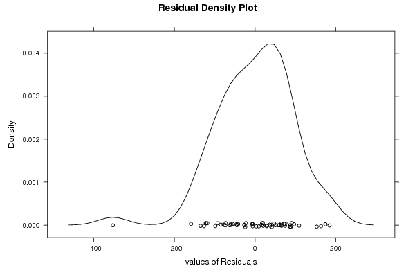
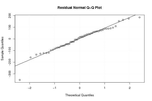
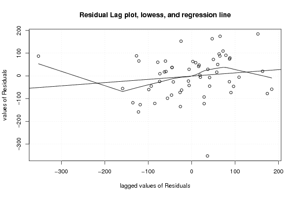
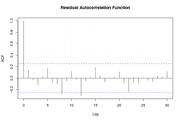
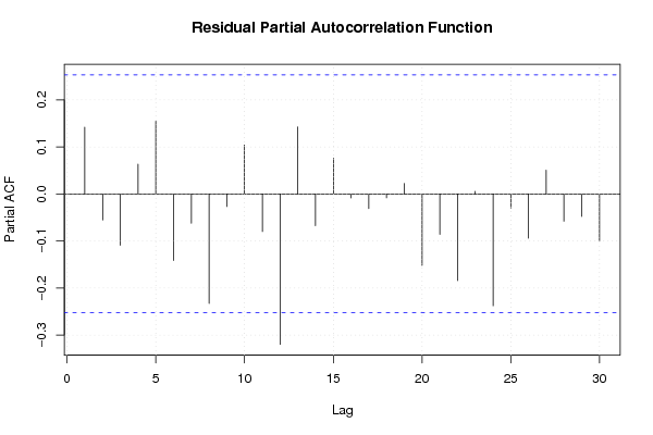
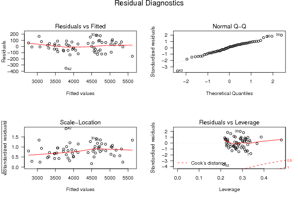
Charts produced by software:

http://www.freestatistics.org/blog/date/2011/Feb/03/t12967327677r04z1co01m7o8n/10gj2z1296731106.png (open in new window) http://www.freestatistics.org/blog/date/2011/Feb/03/t12967327677r04z1co01m7o8n/10gj2z1296731106.ps (open in new window) http://www.freestatistics.org/blog/date/2011/Feb/03/t12967327677r04z1co01m7o8n/1dnaa1296731106.png (open in new window) http://www.freestatistics.org/blog/date/2011/Feb/03/t12967327677r04z1co01m7o8n/1dnaa1296731106.ps (open in new window) http://www.freestatistics.org/blog/date/2011/Feb/03/t12967327677r04z1co01m7o8n/2eu7x1296731106.png (open in new window) http://www.freestatistics.org/blog/date/2011/Feb/03/t12967327677r04z1co01m7o8n/2eu7x1296731106.ps (open in new window) http://www.freestatistics.org/blog/date/2011/Feb/03/t12967327677r04z1co01m7o8n/360sy1296731106.png (open in new window) http://www.freestatistics.org/blog/date/2011/Feb/03/t12967327677r04z1co01m7o8n/360sy1296731106.ps (open in new window) http://www.freestatistics.org/blog/date/2011/Feb/03/t12967327677r04z1co01m7o8n/4zv381296731106.png (open in new window) http://www.freestatistics.org/blog/date/2011/Feb/03/t12967327677r04z1co01m7o8n/4zv381296731106.ps (open in new window) http://www.freestatistics.org/blog/date/2011/Feb/03/t12967327677r04z1co01m7o8n/5kdc91296731106.png (open in new window) http://www.freestatistics.org/blog/date/2011/Feb/03/t12967327677r04z1co01m7o8n/5kdc91296731106.ps (open in new window) http://www.freestatistics.org/blog/date/2011/Feb/03/t12967327677r04z1co01m7o8n/6txy21296731106.png (open in new window) http://www.freestatistics.org/blog/date/2011/Feb/03/t12967327677r04z1co01m7o8n/6txy21296731106.ps (open in new window) http://www.freestatistics.org/blog/date/2011/Feb/03/t12967327677r04z1co01m7o8n/7hdrz1296731106.png (open in new window) http://www.freestatistics.org/blog/date/2011/Feb/03/t12967327677r04z1co01m7o8n/7hdrz1296731106.ps (open in new window) http://www.freestatistics.org/blog/date/2011/Feb/03/t12967327677r04z1co01m7o8n/88s2f1296731106.png (open in new window) http://www.freestatistics.org/blog/date/2011/Feb/03/t12967327677r04z1co01m7o8n/88s2f1296731106.ps (open in new window) http://www.freestatistics.org/blog/date/2011/Feb/03/t12967327677r04z1co01m7o8n/96hqi1296731106.png (open in new window) http://www.freestatistics.org/blog/date/2011/Feb/03/t12967327677r04z1co01m7o8n/96hqi1296731106.ps (open in new window)

Parameters (Session):

par1 = 1 ; par2 = Include Monthly Dummies ; par3 = Linear Trend ;

Parameters (R input):

par1 = 1 ; par2 = Include Monthly Dummies ; par3 = Linear Trend ;

R code (references can be found in the software module):

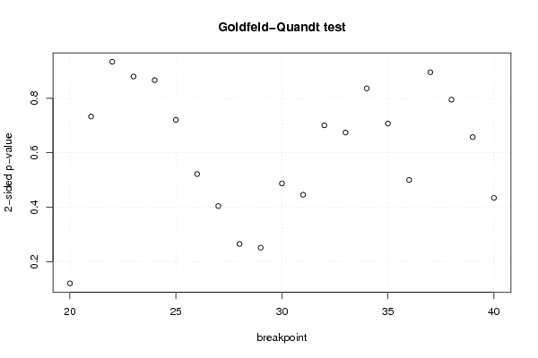
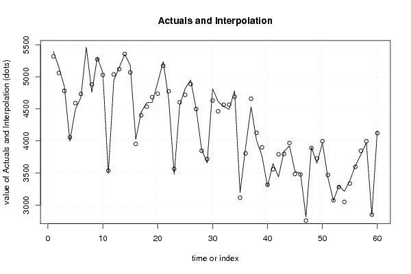
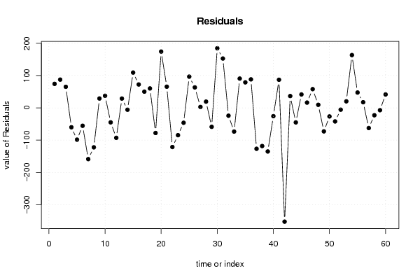
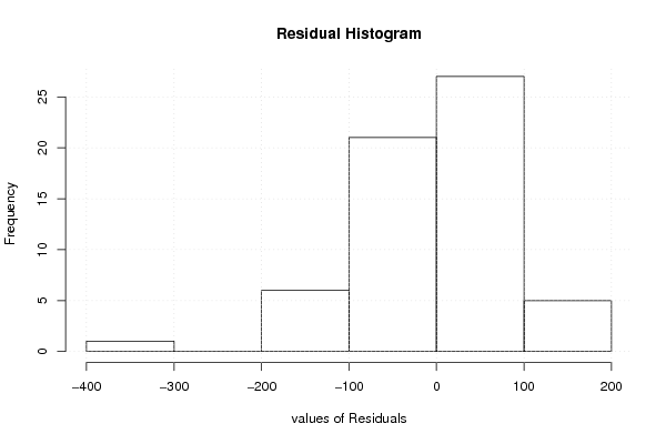
library(lattice) library(lmtest) n25 <- 25 #minimum number of obs. for Goldfeld-Quandt test par1 <- as.numeric(par1) x <- t(y) k <- length(x[1,]) n <- length(x[,1]) x1 <- cbind(x[,par1], x[,1:k!=par1]) mycolnames <- c(colnames(x)[par1], colnames(x)[1:k!=par1]) colnames(x1) <- mycolnames #colnames(x)[par1] x <- x1 if (par3 == 'First Differences'){ x2 <- array(0, dim=c(n-1,k), dimnames=list(1:(n-1), paste('(1-B)',colnames(x),sep=''))) for (i in 1:n-1) { for (j in 1:k) { x2[i,j] <- x[i+1,j] - x[i,j] } } x <- x2 } if (par2 == 'Include Monthly Dummies'){ x2 <- array(0, dim=c(n,11), dimnames=list(1:n, paste('M', seq(1:11), sep =''))) for (i in 1:11){ x2[seq(i,n,12),i] <- 1 } x <- cbind(x, x2) } if (par2 == 'Include Quarterly Dummies'){ x2 <- array(0, dim=c(n,3), dimnames=list(1:n, paste('Q', seq(1:3), sep =''))) for (i in 1:3){ x2[seq(i,n,4),i] <- 1 } x <- cbind(x, x2) } k <- length(x[1,]) if (par3 == 'Linear Trend'){ x <- cbind(x, c(1:n)) colnames(x)[k+1] <- 't' } x k <- length(x[1,]) df <- as.data.frame(x) (mylm <- lm(df)) (mysum <- summary(mylm)) if (n > n25) { kp3 <- k + 3 nmkm3 <- n - k - 3 gqarr <- array(NA, dim=c(nmkm3-kp3+1,3)) numgqtests <- 0 numsignificant1 <- 0 numsignificant5 <- 0 numsignificant10 <- 0 for (mypoint in kp3:nmkm3) { j <- 0 numgqtests <- numgqtests + 1 for (myalt in c('greater', 'two.sided', 'less')) { j <- j + 1 gqarr[mypoint-kp3+1,j] <- gqtest(mylm, point=mypoint, alternative=myalt)$p.value } if (gqarr[mypoint-kp3+1,2] < 0.01) numsignificant1 <- numsignificant1 + 1 if (gqarr[mypoint-kp3+1,2] < 0.05) numsignificant5 <- numsignificant5 + 1 if (gqarr[mypoint-kp3+1,2] < 0.10) numsignificant10 <- numsignificant10 + 1 } gqarr } bitmap(file='test0.png') plot(x[,1], type='l', main='Actuals and Interpolation', ylab='value of Actuals and Interpolation (dots)', xlab='time or index') points(x[,1]-mysum$resid) grid() dev.off() bitmap(file='test1.png') plot(mysum$resid, type='b', pch=19, main='Residuals', ylab='value of Residuals', xlab='time or index') grid() dev.off() bitmap(file='test2.png') hist(mysum$resid, main='Residual Histogram', xlab='values of Residuals') grid() dev.off() bitmap(file='test3.png') densityplot(~mysum$resid,col='black',main='Residual Density Plot', xlab='values of Residuals') dev.off() bitmap(file='test4.png') qqnorm(mysum$resid, main='Residual Normal Q-Q Plot') qqline(mysum$resid) grid() dev.off() (myerror <- as.ts(mysum$resid)) bitmap(file='test5.png') dum <- cbind(lag(myerror,k=1),myerror) dum dum1 <- dum[2:length(myerror),] dum1 z <- as.data.frame(dum1) z plot(z,main=paste('Residual Lag plot, lowess, and regression line'), ylab='values of Residuals', xlab='lagged values of Residuals') lines(lowess(z)) abline(lm(z)) grid() dev.off() bitmap(file='test6.png') acf(mysum$resid, lag.max=length(mysum$resid)/2, main='Residual Autocorrelation Function') grid() dev.off() bitmap(file='test7.png') pacf(mysum$resid, lag.max=length(mysum$resid)/2, main='Residual Partial Autocorrelation Function') grid() dev.off() bitmap(file='test8.png') opar <- par(mfrow = c(2,2), oma = c(0, 0, 1.1, 0)) plot(mylm, las = 1, sub='Residual Diagnostics') par(opar) dev.off() if (n > n25) { bitmap(file='test9.png') plot(kp3:nmkm3,gqarr[,2], main='Goldfeld-Quandt test',ylab='2-sided p-value',xlab='breakpoint') grid() dev.off() } load(file='createtable') a<-table.start() a<-table.row.start(a) a<-table.element(a, 'Multiple Linear Regression - Estimated Regression Equation', 1, TRUE) a<-table.row.end(a) myeq <- colnames(x)[1] myeq <- paste(myeq, '[t] = ', sep='') for (i in 1:k){ if (mysum$coefficients[i,1] > 0) myeq <- paste(myeq, '+', '') myeq <- paste(myeq, mysum$coefficients[i,1], sep=' ') if (rownames(mysum$coefficients)[i] != '(Intercept)') { myeq <- paste(myeq, rownames(mysum$coefficients)[i], sep='') if (rownames(mysum$coefficients)[i] != 't') myeq <- paste(myeq, '[t]', sep='') } } myeq <- paste(myeq, ' + e[t]') a<-table.row.start(a) a<-table.element(a, myeq) a<-table.row.end(a) a<-table.end(a) table.save(a,file='mytable1.tab') a<-table.start() a<-table.row.start(a) a<-table.element(a,hyperlink('http://www.xycoon.com/ols1.htm','Multiple Linear Regression - Ordinary Least Squares',''), 6, TRUE) a<-table.row.end(a) a<-table.row.start(a) a<-table.element(a,'Variable',header=TRUE) a<-table.element(a,'Parameter',header=TRUE) a<-table.element(a,'S.D.',header=TRUE) a<-table.element(a,'T-STAT<br />H0: parameter = 0',header=TRUE) a<-table.element(a,'2-tail p-value',header=TRUE) a<-table.element(a,'1-tail p-value',header=TRUE) a<-table.row.end(a) for (i in 1:k){ a<-table.row.start(a) a<-table.element(a,rownames(mysum$coefficients)[i],header=TRUE) a<-table.element(a,mysum$coefficients[i,1]) a<-table.element(a, round(mysum$coefficients[i,2],6)) a<-table.element(a, round(mysum$coefficients[i,3],4)) a<-table.element(a, round(mysum$coefficients[i,4],6)) a<-table.element(a, round(mysum$coefficients[i,4]/2,6)) a<-table.row.end(a) } a<-table.end(a) table.save(a,file='mytable2.tab') a<-table.start() a<-table.row.start(a) a<-table.element(a, 'Multiple Linear Regression - Regression Statistics', 2, TRUE) a<-table.row.end(a) a<-table.row.start(a) a<-table.element(a, 'Multiple R',1,TRUE) a<-table.element(a, sqrt(mysum$r.squared)) a<-table.row.end(a) a<-table.row.start(a) a<-table.element(a, 'R-squared',1,TRUE) a<-table.element(a, mysum$r.squared) a<-table.row.end(a) a<-table.row.start(a) a<-table.element(a, 'Adjusted R-squared',1,TRUE) a<-table.element(a, mysum$adj.r.squared) a<-table.row.end(a) a<-table.row.start(a) a<-table.element(a, 'F-TEST (value)',1,TRUE) a<-table.element(a, mysum$fstatistic[1]) a<-table.row.end(a) a<-table.row.start(a) a<-table.element(a, 'F-TEST (DF numerator)',1,TRUE) a<-table.element(a, mysum$fstatistic[2]) a<-table.row.end(a) a<-table.row.start(a) a<-table.element(a, 'F-TEST (DF denominator)',1,TRUE) a<-table.element(a, mysum$fstatistic[3]) a<-table.row.end(a) a<-table.row.start(a) a<-table.element(a, 'p-value',1,TRUE) a<-table.element(a, 1-pf(mysum$fstatistic[1],mysum$fstatistic[2],mysum$fstatistic[3])) a<-table.row.end(a) a<-table.row.start(a) a<-table.element(a, 'Multiple Linear Regression - Residual Statistics', 2, TRUE) a<-table.row.end(a) a<-table.row.start(a) a<-table.element(a, 'Residual Standard Deviation',1,TRUE) a<-table.element(a, mysum$sigma) a<-table.row.end(a) a<-table.row.start(a) a<-table.element(a, 'Sum Squared Residuals',1,TRUE) a<-table.element(a, sum(myerror*myerror)) a<-table.row.end(a) a<-table.end(a) table.save(a,file='mytable3.tab') a<-table.start() a<-table.row.start(a) a<-table.element(a, 'Multiple Linear Regression - Actuals, Interpolation, and Residuals', 4, TRUE) a<-table.row.end(a) a<-table.row.start(a) a<-table.element(a, 'Time or Index', 1, TRUE) a<-table.element(a, 'Actuals', 1, TRUE) a<-table.element(a, 'Interpolation<br />Forecast', 1, TRUE) a<-table.element(a, 'Residuals<br />Prediction Error', 1, TRUE) a<-table.row.end(a) for (i in 1:n) { a<-table.row.start(a) a<-table.element(a,i, 1, TRUE) a<-table.element(a,x[i]) a<-table.element(a,x[i]-mysum$resid[i]) a<-table.element(a,mysum$resid[i]) a<-table.row.end(a) } a<-table.end(a) table.save(a,file='mytable4.tab') if (n > n25) { a<-table.start() a<-table.row.start(a) a<-table.element(a,'Goldfeld-Quandt test for Heteroskedasticity',4,TRUE) a<-table.row.end(a) a<-table.row.start(a) a<-table.element(a,'p-values',header=TRUE) a<-table.element(a,'Alternative Hypothesis',3,header=TRUE) a<-table.row.end(a) a<-table.row.start(a) a<-table.element(a,'breakpoint index',header=TRUE) a<-table.element(a,'greater',header=TRUE) a<-table.element(a,'2-sided',header=TRUE) a<-table.element(a,'less',header=TRUE) a<-table.row.end(a) for (mypoint in kp3:nmkm3) { a<-table.row.start(a) a<-table.element(a,mypoint,header=TRUE) a<-table.element(a,gqarr[mypoint-kp3+1,1]) a<-table.element(a,gqarr[mypoint-kp3+1,2]) a<-table.element(a,gqarr[mypoint-kp3+1,3]) a<-table.row.end(a) } a<-table.end(a) table.save(a,file='mytable5.tab') a<-table.start() a<-table.row.start(a) a<-table.element(a,'Meta Analysis of Goldfeld-Quandt test for Heteroskedasticity',4,TRUE) a<-table.row.end(a) a<-table.row.start(a) a<-table.element(a,'Description',header=TRUE) a<-table.element(a,'# significant tests',header=TRUE) a<-table.element(a,'% significant tests',header=TRUE) a<-table.element(a,'OK/NOK',header=TRUE) a<-table.row.end(a) a<-table.row.start(a) a<-table.element(a,'1% type I error level',header=TRUE) a<-table.element(a,numsignificant1) a<-table.element(a,numsignificant1/numgqtests) if (numsignificant1/numgqtests < 0.01) dum <- 'OK' else dum <- 'NOK' a<-table.element(a,dum) a<-table.row.end(a) a<-table.row.start(a) a<-table.element(a,'5% type I error level',header=TRUE) a<-table.element(a,numsignificant5) a<-table.element(a,numsignificant5/numgqtests) if (numsignificant5/numgqtests < 0.05) dum <- 'OK' else dum <- 'NOK' a<-table.element(a,dum) a<-table.row.end(a) a<-table.row.start(a) a<-table.element(a,'10% type I error level',header=TRUE) a<-table.element(a,numsignificant10) a<-table.element(a,numsignificant10/numgqtests) if (numsignificant10/numgqtests < 0.1) dum <- 'OK' else dum <- 'NOK' a<-table.element(a,dum) a<-table.row.end(a) a<-table.end(a) table.save(a,file='mytable6.tab') }

Copyright

This work is licensed under a Creative Commons Attribution-Noncommercial-Share Alike 3.0 License.

Software written by Ed van Stee & Patrick Wessa

Disclaimer

Information provided on this web site is provided "AS IS" without warranty of any kind, either express or implied, including, without limitation, warranties of merchantability, fitness for a particular purpose, and noninfringement. We use reasonable efforts to include accurate and timely information and periodically update the information, and software without notice. However, we make no warranties or representations as to the accuracy or completeness of such information (or software), and we assume no liability or responsibility for errors or omissions in the content of this web site, or any software bugs in online applications. Your use of this web site is AT YOUR OWN RISK. Under no circumstances and under no legal theory shall we be liable to you or any other person for any direct, indirect, special, incidental, exemplary, or consequential damages arising from your access to, or use of, this web site.

Privacy Policy

We may request personal information to be submitted to our servers in order to be able to:

• personalize online software applications according to your needs
• enforce strict security rules with respect to the data that you upload (e.g. statistical data)
• manage user sessions of online applications
• alert you about important changes or upgrades in resources or applications

We NEVER allow other companies to directly offer registered users information about their products and services. Banner references and hyperlinks of third parties NEVER contain any personal data of the visitor.

We do NOT sell, nor transmit by any means, personal information, nor statistical data series uploaded by you to third parties.

We carefully protect your data from loss, misuse, alteration, and destruction. However, at any time, and under any circumstance you are solely responsible for managing your passwords, and keeping them secret.

We store a unique ANONYMOUS USER ID in the form of a small 'Cookie' on your computer. This allows us to track your progress when using this website which is necessary to create state-dependent features. The cookie is used for NO OTHER PURPOSE. At any time you may opt to disallow cookies from this website - this will not affect other features of this website.

We examine cookies that are used by third-parties (banner and online ads) very closely: abuse from third-parties automatically results in termination of the advertising contract without refund. We have very good reason to believe that the cookies that are produced by third parties (banner ads) do NOT cause any privacy or security risk.

FreeStatistics.org is safe. There is no need to download any software to use the applications and services contained in this website. Hence, your system's security is not compromised by their use, and your personal data - other than data you submit in the account application form, and the user-agent information that is transmitted by your browser - is never transmitted to our servers.

As a general rule, we do not log on-line behavior of individuals (other than normal logging of webserver 'hits'). However, in cases of abuse, hacking, unauthorized access, Denial of Service attacks, illegal copying, hotlinking, non-compliance with international webstandards (such as robots.txt), or any other harmful behavior, our system engineers are empowered to log, track, identify, publish, and ban misbehaving individuals - even if this leads to ban entire blocks of IP addresses, or disclosing user's identity.

FreeStatistics.org is powered by