Free Statistics

of Irreproducible Research!

Author's title

Author*Unverified author*
R Software Modulerwasp_icvl2008.wasp
Title produced by softwareInternational Conference on Virtual Learning 2008
Date of computationMon, 30 Jun 2008 09:51:50 -0600
Cite this page as followsStatistical Computations at FreeStatistics.org, Office for Research Development and Education, URL https://freestatistics.org/blog/index.php?v=date/2008/Jun/30/t1214841152sn6jlyhgseclgqm.htm/, Retrieved Thu, 28 Mar 2024 08:47:41 +0000
Statistical Computations at FreeStatistics.org, Office for Research Development and Education, URL https://freestatistics.org/blog/index.php?pk=13777, Retrieved Thu, 28 Mar 2024 08:47:41 +0000
QR Codes:

Original text written by user:
IsPrivate?No (this computation is public)
User-defined keywords
Estimated Impact560
Family? (F = Feedback message, R = changed R code, M = changed R Module, P = changed Parameters, D = changed Data)
-       [International Conference on Virtual Learning 2008] [ICVL 2008 - Figure 3] [2008-06-30 15:51:50] [d41d8cd98f00b204e9800998ecf8427e] [Current]
Feedback Forum

Post a new message


Summary of computational transaction
Raw Inputview raw input (R code)
Raw Outputview raw output of R engine
Computing time11 seconds
R Server'Herman Ole Andreas Wold' @ 193.190.124.10:1001

\begin{tabular}{lllllllll}
\hline
Summary of computational transaction \tabularnewline
Raw Input & view raw input (R code)  \tabularnewline
Raw Output & view raw output of R engine  \tabularnewline
Computing time & 11 seconds \tabularnewline
R Server & 'Herman Ole Andreas Wold' @ 193.190.124.10:1001 \tabularnewline
\hline
\end{tabular}
%Source: https://freestatistics.org/blog/index.php?pk=13777&T=0

[TABLE]
[ROW][C]Summary of computational transaction[/C][/ROW]
[ROW][C]Raw Input[/C][C]view raw input (R code) [/C][/ROW]
[ROW][C]Raw Output[/C][C]view raw output of R engine [/C][/ROW]
[ROW][C]Computing time[/C][C]11 seconds[/C][/ROW]
[ROW][C]R Server[/C][C]'Herman Ole Andreas Wold' @ 193.190.124.10:1001[/C][/ROW]
[/TABLE]
Source: https://freestatistics.org/blog/index.php?pk=13777&T=0

Globally Unique Identifier (entire table): ba.freestatistics.org/blog/index.php?pk=13777&T=0

As an alternative you can also use a QR Code:  

The GUIDs for individual cells are displayed in the table below:

Summary of computational transaction
Raw Inputview raw input (R code)
Raw Outputview raw output of R engine
Computing time11 seconds
R Server'Herman Ole Andreas Wold' @ 193.190.124.10:1001


Correlations between reported intention to use and # reproducible computations
Pearson rhoPearson p-valueKendall tauKendall p-value
Female Bachelor Students-0.080.5507-0.08540.3783
Male Bachelor Students-0.14530.2992-0.11710.2547
Female Switching Students0.01610.90910.03110.763
Male Switching Students0.24160.03550.1710.0416

\begin{tabular}{lllllllll}
\hline
Correlations between reported intention to use and # reproducible computations \tabularnewline
 & Pearson rho & Pearson p-value & Kendall tau & Kendall p-value \tabularnewline
Female Bachelor Students & -0.08 & 0.5507 & -0.0854 & 0.3783 \tabularnewline
Male Bachelor Students & -0.1453 & 0.2992 & -0.1171 & 0.2547 \tabularnewline
Female Switching Students & 0.0161 & 0.9091 & 0.0311 & 0.763 \tabularnewline
Male Switching Students & 0.2416 & 0.0355 & 0.171 & 0.0416 \tabularnewline
\hline
\end{tabular}
%Source: https://freestatistics.org/blog/index.php?pk=13777&T=1

[TABLE]
[ROW][C]Correlations between reported intention to use and # reproducible computations[/C][/ROW]
[ROW][C][/C][C]Pearson rho[/C][C]Pearson p-value[/C][C]Kendall tau[/C][C]Kendall p-value[/C][/ROW]
[ROW][C]Female Bachelor Students[/C][C]-0.08[/C][C]0.5507[/C][C]-0.0854[/C][C]0.3783[/C][/ROW]
[ROW][C]Male Bachelor Students[/C][C]-0.1453[/C][C]0.2992[/C][C]-0.1171[/C][C]0.2547[/C][/ROW]
[ROW][C]Female Switching Students[/C][C]0.0161[/C][C]0.9091[/C][C]0.0311[/C][C]0.763[/C][/ROW]
[ROW][C]Male Switching Students[/C][C]0.2416[/C][C]0.0355[/C][C]0.171[/C][C]0.0416[/C][/ROW]
[/TABLE]
Source: https://freestatistics.org/blog/index.php?pk=13777&T=1

Globally Unique Identifier (entire table): ba.freestatistics.org/blog/index.php?pk=13777&T=1

As an alternative you can also use a QR Code:  

The GUIDs for individual cells are displayed in the table below:

Correlations between reported intention to use and # reproducible computations
Pearson rhoPearson p-valueKendall tauKendall p-value
Female Bachelor Students-0.080.5507-0.08540.3783
Male Bachelor Students-0.14530.2992-0.11710.2547
Female Switching Students0.01610.90910.03110.763
Male Switching Students0.24160.03550.1710.0416


Parameters (Session):
par1 = reported computing ; par2 = actual computing ;
Parameters (R input):
par1 = reported computing ; par2 = actual computing ;
R code (references can be found in the software module):
x <- as.data.frame(read.table(file='https://automated.biganalytics.eu/download/statdb.csv',sep=',',header=T))
library(GenKern)
load(file='createtable')
doplot1 <- function(myxcol,myycol,myxlab='',myylab='') {
p0 <- x[x$Pop==0,]
p1 <- x[x$Pop==1,]
dum <- cbind(p0[,myxcol],rank(p0[,myxcol]),p0[,'Gender'])
xf0 <- dum[dum[,3]==0,2]
xm0 <- dum[dum[,3]==1,2]
dum <- cbind(p0[,myycol],rank(p0[,myycol]),p0[,'Gender'])
yf0 <- dum[dum[,3]==0,2]
ym0 <- dum[dum[,3]==1,2]
dum <- cbind(p1[,myxcol],rank(p1[,myxcol]),p1[,'Gender'])
xf1 <- dum[dum[,3]==0,2]
xm1 <- dum[dum[,3]==1,2]
dum <- cbind(p1[,myycol],rank(p1[,myycol]),p1[,'Gender'])
yf1 <- dum[dum[,3]==0,2]
ym1 <- dum[dum[,3]==1,2]
xf <- rank(x[x$Gender==0,myxcol])
yf <- rank(x[x$Gender==0,myycol])
xm <- rank(x[x$Gender==1,myxcol])
ym <- rank(x[x$Gender==1,myycol])
x0 <- rank(x[x$Pop==0,myxcol])
y0 <- rank(x[x$Pop==0,myycol])
x1 <- rank(x[x$Pop==1,myxcol])
y1 <- rank(x[x$Pop==1,myycol])
mycorr <- array(NA,dim=c(4,4))
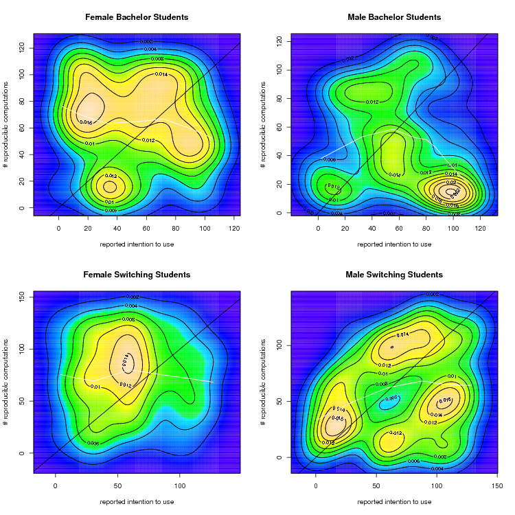
rownames(mycorr) <- c('Female Bachelor Students','Male Bachelor Students','Female Switching Students','Male Switching Students')
colnames(mycorr) <- c('Pearson rho','Pearson p-value','Kendall tau','Kendall p-value')
bitmap(file='mypicture.png')
par(mfrow=c(2,2))
r <- cor.test(xf0,yf0,method='pearson')
mycorr[1,1] <- r$estimate
mycorr[1,2] <- r$p.value
r <- cor.test(xf0,yf0,method='kendall')
mycorr[1,3] <- r$estimate
mycorr[1,4] <- r$p.value
op <- KernSur(xf0,yf0, xgridsize=150, ygridsize=150,na.rm=T)
image(op$xords, op$yords, op$zden, col=topo.colors(100), axes=TRUE, xlab=myxlab, ylab=myylab, main=rownames(mycorr)[1])
contour(op$xords, op$yords, op$zden, add=TRUE)
box()
abline(0,1)
lines(stats::lowess(cbind(xf0,yf0)),col='white')
r <- cor.test(xm0,ym0,method='pearson')
mycorr[2,1] <- r$estimate
mycorr[2,2] <- r$p.value
r <- cor.test(xm0,ym0,method='kendall')
mycorr[2,3] <- r$estimate
mycorr[2,4] <- r$p.value
op <- KernSur(xm0,ym0, xgridsize=150, ygridsize=150,na.rm=T)
image(op$xords, op$yords, op$zden, col=topo.colors(100), axes=TRUE, xlab=myxlab, ylab=myylab, main=rownames(mycorr)[2])
contour(op$xords, op$yords, op$zden, add=TRUE)
box()
abline(0,1)
lines(stats::lowess(cbind(xm0,ym0)),col='white')
r <- cor.test(xf1,yf1,method='pearson')
mycorr[3,1] <- r$estimate
mycorr[3,2] <- r$p.value
r <- cor.test(xf1,yf1,method='kendall')
mycorr[3,3] <- r$estimate
mycorr[3,4] <- r$p.value
op <- KernSur(xf1,yf1, xgridsize=150, ygridsize=150,na.rm=T)
image(op$xords, op$yords, op$zden, col=topo.colors(100), axes=TRUE, xlab=myxlab, ylab=myylab, main=rownames(mycorr)[3])
contour(op$xords, op$yords, op$zden, add=TRUE)
box()
abline(0,1)
lines(stats::lowess(cbind(xf1,yf1)),col='white')
r <- cor.test(xm1,ym1,method='pearson')
mycorr[4,1] <- r$estimate
mycorr[4,2] <- r$p.value
r <- cor.test(xm1,ym1,method='kendall')
mycorr[4,3] <- r$estimate
mycorr[4,4] <- r$p.value
op <- KernSur(xm1,ym1, xgridsize=150, ygridsize=150,na.rm=T)
image(op$xords, op$yords, op$zden, col=topo.colors(100), axes=TRUE, xlab=myxlab, ylab=myylab, main=rownames(mycorr)[4])
contour(op$xords, op$yords, op$zden, add=TRUE)
box()
abline(0,1)
lines(stats::lowess(cbind(xm1,ym1)),col='white')
dev.off()
mycorr
}
if (par1 == 'actual feedback') {
myxcol='nnzfg'
myxlab = '# submitted messages'
}
if (par1 == 'reported feedback') {
myxcol = 'Reflection'
myxlab = 'reported feedback submissions'
}
if (par1 == 'reported computing') {
myxcol = 'Future'
myxlab = 'reported intention to use'
}
if (par2 == 'actual computing') {
myycol = 'Bcount'
myylab = '# reproducible computations'
}
if (par2 == 'actual feedback') {
myycol = 'nnzfg'
myylab = 'actual feedback submissions'
}
if (par2 == 'reported computing') {
myycol = 'Future'
myylab = 'reported intention to use'
}
mycorr <- doplot1(myxcol=myxcol,myycol=myycol,myxlab=myxlab,myylab=myylab)
a<-table.start()
a<-table.row.start(a)
dum <- 'Correlations between'
dum <- paste(dum,myxlab,sep=' ')
dum <- paste(dum,myylab,sep=' and ')
a<-table.element(a,dum,5,TRUE)
a<-table.row.end(a)
a<-table.row.start(a)
a<-table.element(a,'',header=TRUE)
a<-table.element(a,'Pearson rho',header=TRUE)
a<-table.element(a,'Pearson p-value',header=TRUE)
a<-table.element(a,'Kendall tau',header=TRUE)
a<-table.element(a,'Kendall p-value',header=TRUE)
a<-table.row.end(a)
for (myrow in 1:4) {
a<-table.row.start(a)
a<-table.element(a,rownames(mycorr)[myrow],header=TRUE)
a<-table.element(a,round(mycorr[myrow,1],4))
a<-table.element(a,round(mycorr[myrow,2],4))
a<-table.element(a,round(mycorr[myrow,3],4))
a<-table.element(a,round(mycorr[myrow,4],4))
a<-table.row.end(a)
}
a<-table.end(a)
table.save(a,file='mytable.tab')