serrsBayes provides model-based quantification of
surface-enhanced resonance Raman spectroscopy (SERRS) using sequential
Monte Carlo (SMC) algorithms. The details of the Bayesian model and
informative priors are provided in Moores et al. (2026) “Bayesian
modelling and quantification of Raman spectroscopy.,” published in
the 2025 MATRIX Annals, Part II (Springer). Development of this
software was supported by the UK Engineering & Physical Sciences
Research Council (EPSRC) programme grant “In Situ
Nanoparticle Assemblies for Healthcare Diagnostics and Therapy”
(ref: EP/L014165/1).
Stable releases, including binary packages for Windows & Mac OS, are available from CRAN:
install.packages("serrsBayes")The current development version can be installed from GitHub:
devtools::install_github("mooresm/serrsBayes")To simulate a synthetic Raman spectrum with known parameters:
set.seed(1234)
library(serrsBayes)

wavenumbers <- seq(700,1400,by=2)
spectra <- matrix(nrow=1, ncol=length(wavenumbers))
peakLocations <- c(840,  960, 1140, 1220, 1290)
peakAmplitude <- c(11500, 2500, 4000, 3000, 2500)
peakScale <- c(10, 15, 20, 10, 12)
signature <- weightedLorentzian(peakLocations, peakScale, peakAmplitude, wavenumbers)
baseline <- 1000*cos(wavenumbers/200) + 2*wavenumbers
spectra[1,] <- signature + baseline + rnorm(length(wavenumbers),0,200)
plot(wavenumbers, spectra[1,], type='l', xlab=expression(paste("Raman shift (cm"^{-1}, ")")), ylab="Intensity (a.u.)")
lines(wavenumbers, baseline, col=2, lty=4)
lines(wavenumbers, baseline + signature, col=4, lty=2, lwd=2)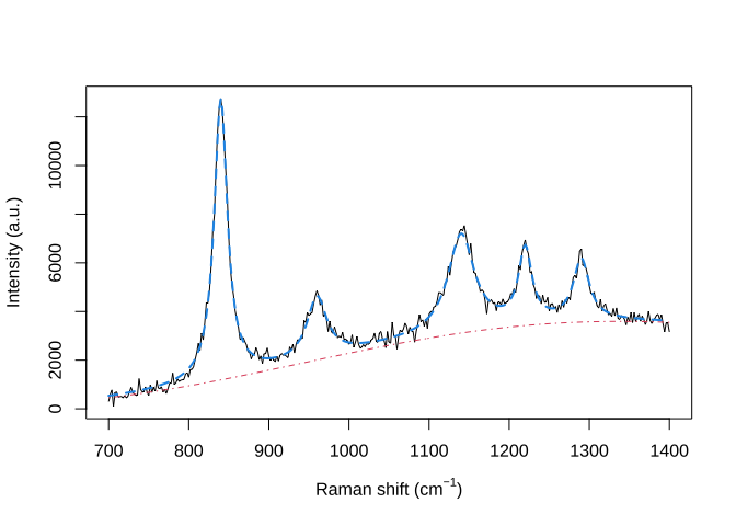
Fit the model using SMC:
lPriors <- list(scale.mu=log(11.6) - (0.4^2)/2, scale.sd=0.4, bl.smooth=10^11, bl.knots=50,
                 beta.mu=5000, beta.sd=5000, noise.sd=200, noise.nu=4)
tm <- system.time(result <- fitSpectraSMC(wavenumbers, spectra, peakLocations, lPriors))
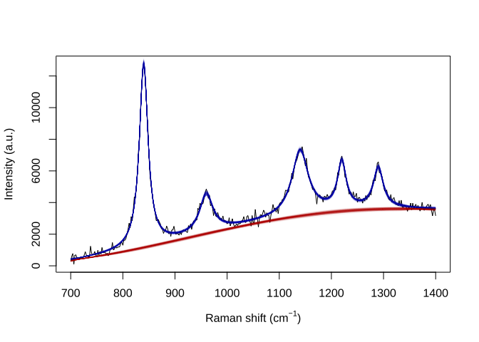
Sample 200 particles from the posterior distribution:
print(tm)
#>    user  system elapsed
#> 164.263   1.925  43.341
samp.idx <- sample.int(length(result$weights), 200, prob=result$weights)
plot(wavenumbers, spectra[1,], type='l', xlab=expression(paste("Raman shift (cm"^{-1}, ")")), ylab="Intensity (a.u.)")
for (pt in samp.idx) {
  bl.est <- result$basis %*% result$alpha[,1,pt]
  lines(wavenumbers, bl.est, col="#C3000009")
  lines(wavenumbers, bl.est + result$expFn[pt,], col="#0000C309")
}