orbitr

Tidy N-body orbital mechanics for R.

Version 1.0 — the function names, arguments, and defaults are now stable; anything that changes in a future version will be deprecated first. Feedback, bug reports, and contributions are welcome on GitHub.

Full documentation, examples, and guides at orbit-r.com

Installation

# Install from CRAN:
install.packages("orbitr")

# Or install the development version from GitHub:
# install.packages("devtools")
devtools::install_github("DRosenman/orbitr")

The Full Solar System in A Few Lines

library(orbitr)

load_solar_system() |>
  simulate_system(time_step = seconds_per_day, duration = seconds_per_year) |>
  plot_orbits(three_d = FALSE)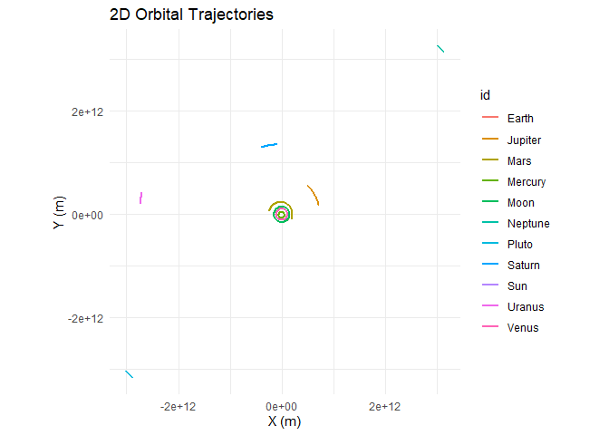

load_solar_system() builds the Sun, all eight planets, the Moon, and Pluto with real orbital data from JPL — eccentricities, inclinations, and all. One line to build it, one line to simulate and plot.

Don’t need every body? Drop them with remove_body():

load_solar_system() |>
  remove_body(c("Pluto", "Moon")) |>
  simulate_system(time_step = seconds_per_day, duration = seconds_per_year) |>
  plot_orbits(three_d = FALSE)

Four Lines to an Orbit

library(orbitr)

sim <- create_system() |>
  add_sun() |>
  add_body("Earth", mass = mass_earth, x = distance_earth_sun, vy = speed_earth) |>
  simulate_system(time_step = seconds_per_day, duration = seconds_per_year)

sim |> plot_orbits()

Built-in constants like mass_sun, distance_earth_sun, and speed_earth are real-world values in SI units — no Googling needed. simulate_system() returns a tidy tibble, ready for dplyr, ggplot2, plotly, or anything else.

Animated

animate_system(sim, fps = 15, duration = 5)

More Examples

Build Your Own System with add_planet()

Pick and choose real solar system bodies without looking up any numbers:

create_system() |>
  add_sun() |>
  add_planet("Earth", parent = "Sun") |>
  add_planet("Mars",  parent = "Sun") |>
  simulate_system(time_step = seconds_per_day, duration = seconds_per_year * 2) |>
  plot_orbits(three_d = FALSE)

Every planet’s mass, eccentricity, inclination, and orbital orientation are filled in from JPL data. Override any element to explore “what if” scenarios:

# What if Mars had a perfectly circular orbit?
create_system() |>
  add_sun() |>
  add_planet("Mars", parent = "Sun", e = 0) |>
  simulate_system(time_step = seconds_per_day, duration = seconds_per_year * 2) |>
  plot_orbits(three_d = FALSE)

Earth-Moon

create_system() |>
  add_body("Earth", mass = mass_earth) |>
  add_planet("Moon", parent = "Earth") |>
  simulate_system(time_step = seconds_per_hour, duration = seconds_per_day * 28) |>
  plot_orbits()

Keplerian Orbital Elements

For full control, add_body_keplerian() lets you specify orbits using classical elements — semi-major axis, eccentricity, inclination, and orientation angles — instead of raw positions and velocities:

# A comet on a highly eccentric, tilted orbit
create_system() |>
  add_sun() |>
  add_planet("Earth", parent = "Sun") |>
  add_body_keplerian(
    "Comet", mass = 1e13, parent = "Sun",
    a = 3 * distance_earth_sun, e = 0.85,
    i = 60, lan = 45, arg_pe = 90, nu = 0
  ) |>
  simulate_system(time_step = seconds_per_hour, duration = seconds_per_year * 5) |>
  plot_orbits()

Kepler-16: A Real Circumbinary Planet

Kepler-16b orbits two stars — a real-life Tatooine.

G  <- gravitational_constant
AU <- distance_earth_sun

m_A <- 0.68 * mass_sun
m_B <- 0.20 * mass_sun
a_bin <- 0.22 * AU

r_A <- a_bin * m_B / (m_A + m_B)
r_B <- a_bin * m_A / (m_A + m_B)
v_A <- sqrt(G * m_B^2 / ((m_A + m_B) * a_bin))
v_B <- sqrt(G * m_A^2 / ((m_A + m_B) * a_bin))

r_planet <- 0.7048 * AU
v_planet <- sqrt(G * (m_A + m_B) / r_planet)

create_system() |>
  add_body("Star A",      mass = m_A,                 x = r_A,      vy = v_A) |>
  add_body("Star B",      mass = m_B,                 x = -r_B,     vy = -v_B) |>
  add_body("Kepler-16b",  mass = 0.333 * mass_jupiter, x = r_planet, vy = v_planet) |>
  simulate_system(time_step = seconds_per_hour, duration = seconds_per_day * 228.8 * 3) |>
  plot_orbits()

Features

• Tidy output — one row per body per time step, works with the whole tidyverse
• Real solar system data — load_solar_system() and add_planet() use JPL orbital elements, no manual setup needed
• Keplerian elements — add_body_keplerian() lets you define orbits with semi-major axis, eccentricity, inclination, and orientation angles
• Built-in constants — masses, distances, and speeds for the Sun, all eight planets, and the Moon
• C++ engine — compiled via Rcpp with automatic fallback to vectorized R
• Three integrators — Velocity Verlet (default), Euler-Cromer, and standard Euler
• 2D and 3D — plot_orbits() auto-dispatches to interactive plotly when any body has Z-axis motion; force either with three_d = TRUE/FALSE
• Animations — animate_system() renders GIFs with fading trails via gganimate
• Reference frames — shift_reference_frame("Earth") re-centers everything on any body, or on the system’s center of mass with "barycenter"
• Orbital elements both ways — add_body_keplerian() builds orbits from elements (including hyperbolic flybys with e > 1); get_orbital_elements() recovers the osculating elements of any body at every time step
• Conservation laws — get_energy(), get_momentum(), and get_angular_momentum() give the system totals at every time step; conserved_quantities() joins them with their errors so you can see whether a run is trustworthy
• Segmented runs — continue_simulation() picks up where a run left off with a different time step, for comets and close encounters
• Save and share — save_system() / load_system() round-trip a system to .rds; export_bodies() writes the body table to CSV

Learn More

• Get Started — full walkthrough
• Building Two-Body Orbits — choosing positions, velocities, and masses
• Keplerian Orbital Elements — the physics behind add_body_keplerian() and add_planet()
• Examples — Earth-Moon, Sun-Earth-Moon, Kepler-16, and more
• The Physics — integrators, softening, and the C++ engine
• Custom Visualization — build your own plots with ggplot2 and plotly
• API Reference — full function documentation
• Interactive Demo — try orbitr in your browser with the Shiny app

Acknowledgments & Further Reading

The physics and numerics in orbitr were informed by Classical Dynamics of Particles and Systems by Thornton & Marion, Computational Physics by Mark Newman, and Data Structures & Algorithms in Python by Canning, Broder & Lafore. The C++ engine was built with help from the official Rcpp documentation on CRAN. See the full Further Reading article for details on how each resource was used.

Shoutout to The College of New Jersey, where I first got hooked on this stuff. Go Lions.

License

MIT