Repository of Reproducible Computations

Free Statistics

of Irreproducible Research!

Author's title

Author

*Unverified author*

R Software Module

rwasp_histogram.wasp

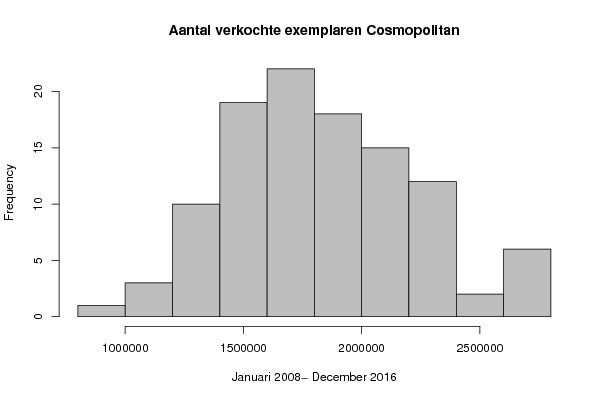
Title produced by software

Histogram

Date of computation

Sun, 30 Jul 2017 21:27:02 +0200

Cite this page as follows

Statistical Computations at FreeStatistics.org, Office for Research Development and Education, URL https://freestatistics.org/blog/index.php?v=date/2017/Jul/30/t1501442839yh2yolr8vym8fn9.htm/, Retrieved Wed, 15 May 2024 12:31:22 +0000

Statistical Computations at FreeStatistics.org, Office for Research Development and Education, URL https://freestatistics.org/blog/index.php?pk=306822, Retrieved Wed, 15 May 2024 12:31:22 +0000

QR Codes:

Paste this QR Code to cite your computation.

Original text written by user:

IsPrivate?

No (this computation is public)

User-defined keywords

Estimated Impact

142

Family? (F = Feedback message, R = changed R code, M = changed R Module, P = changed Parameters, D = changed Data)

-       [Histogram] [] [2017-07-30 19:27:02] [bb1ebaef39f3ee233240b5c77a617fca] [Current]

Feedback Forum

Post a new message

Dataseries X:

Download CSV

Histogram

Boxplots

Summary of computational transaction
Raw Input	view raw input (R code)
Raw Output	view raw output of R engine
Computing time	1 seconds
R Server	Big Analytics Cloud Computing Center

\begin{tabular}{lllllllll}
\hline
Summary of computational transaction \tabularnewline
Raw Input view raw input (R code)  \tabularnewline
Raw Outputview raw output of R engine  \tabularnewline
Computing time1 seconds \tabularnewline
R ServerBig Analytics Cloud Computing Center \tabularnewline
\hline
\end{tabular}
%Source: https://freestatistics.org/blog/index.php?pk=306822&T=0

[TABLE]
[ROW]

Summary of computational transaction[/C][/ROW] [ROW]

Raw Input[/C]

view raw input (R code) [/C][/ROW] [ROW]

Raw Output[/C]

view raw output of R engine [/C][/ROW] [ROW]

Computing time[/C]

1 seconds[/C][/ROW] [ROW]

R Server[/C]

Big Analytics Cloud Computing Center[/C][/ROW] [/TABLE] Source: https://freestatistics.org/blog/index.php?pk=306822&T=0

Globally Unique Identifier (entire table): ba.freestatistics.org/blog/index.php?pk=306822&T=0

As an alternative you can also use a QR Code:

The GUIDs for individual cells are displayed in the table below:

Summary of computational transaction
Raw Input	view raw input (R code)
Raw Output	view raw output of R engine
Computing time	1 seconds
R Server	Big Analytics Cloud Computing Center

Frequency Table (Histogram)
Bins	Midpoint	Abs. Frequency	Rel. Frequency	Cumul. Rel. Freq.	Density
[800000,1000000[	9e+05	1	0.009259	0.009259	0
[1000000,1200000[	1100000	3	0.027778	0.037037	0
[1200000,1400000[	1300000	10	0.092593	0.12963	0
[1400000,1600000[	1500000	19	0.175926	0.305556	1e-06
[1600000,1800000[	1700000	22	0.203704	0.509259	1e-06
[1800000,2000000[	1900000	18	0.166667	0.675926	1e-06
[2000000,2200000[	2100000	15	0.138889	0.814815	1e-06
[2200000,2400000[	2300000	12	0.111111	0.925926	1e-06
[2400000,2600000[	2500000	2	0.018519	0.944444	0
[2600000,2800000]	2700000	6	0.055556	1	0

\begin{tabular}{lllllllll}
\hline
Frequency Table (Histogram) \tabularnewline
Bins & Midpoint & Abs. Frequency & Rel. Frequency & Cumul. Rel. Freq. & Density \tabularnewline
[800000,1000000[ & 9e+05 & 1 & 0.009259 & 0.009259 & 0 \tabularnewline
[1000000,1200000[ & 1100000 & 3 & 0.027778 & 0.037037 & 0 \tabularnewline
[1200000,1400000[ & 1300000 & 10 & 0.092593 & 0.12963 & 0 \tabularnewline
[1400000,1600000[ & 1500000 & 19 & 0.175926 & 0.305556 & 1e-06 \tabularnewline
[1600000,1800000[ & 1700000 & 22 & 0.203704 & 0.509259 & 1e-06 \tabularnewline
[1800000,2000000[ & 1900000 & 18 & 0.166667 & 0.675926 & 1e-06 \tabularnewline
[2000000,2200000[ & 2100000 & 15 & 0.138889 & 0.814815 & 1e-06 \tabularnewline
[2200000,2400000[ & 2300000 & 12 & 0.111111 & 0.925926 & 1e-06 \tabularnewline
[2400000,2600000[ & 2500000 & 2 & 0.018519 & 0.944444 & 0 \tabularnewline
[2600000,2800000] & 2700000 & 6 & 0.055556 & 1 & 0 \tabularnewline
\hline
\end{tabular}
%Source: https://freestatistics.org/blog/index.php?pk=306822&T=1

[TABLE]
[ROW][C]Frequency Table (Histogram)[/C][/ROW]
[ROW][C]Bins[/C][C]Midpoint[/C][C]Abs. Frequency[/C][C]Rel. Frequency[/C][C]Cumul. Rel. Freq.[/C][C]Density[/C][/ROW]
[ROW][C][800000,1000000[[/C][C]9e+05[/C][C]1[/C][C]0.009259[/C][C]0.009259[/C][C]0[/C][/ROW]
[ROW][C][1000000,1200000[[/C][C]1100000[/C][C]3[/C][C]0.027778[/C][C]0.037037[/C][C]0[/C][/ROW]
[ROW][C][1200000,1400000[[/C][C]1300000[/C][C]10[/C][C]0.092593[/C][C]0.12963[/C][C]0[/C][/ROW]
[ROW][C][1400000,1600000[[/C][C]1500000[/C][C]19[/C][C]0.175926[/C][C]0.305556[/C][C]1e-06[/C][/ROW]
[ROW][C][1600000,1800000[[/C][C]1700000[/C][C]22[/C][C]0.203704[/C][C]0.509259[/C][C]1e-06[/C][/ROW]
[ROW][C][1800000,2000000[[/C][C]1900000[/C][C]18[/C][C]0.166667[/C][C]0.675926[/C][C]1e-06[/C][/ROW]
[ROW][C][2000000,2200000[[/C][C]2100000[/C][C]15[/C][C]0.138889[/C][C]0.814815[/C][C]1e-06[/C][/ROW]
[ROW][C][2200000,2400000[[/C][C]2300000[/C][C]12[/C][C]0.111111[/C][C]0.925926[/C][C]1e-06[/C][/ROW]
[ROW][C][2400000,2600000[[/C][C]2500000[/C][C]2[/C][C]0.018519[/C][C]0.944444[/C][C]0[/C][/ROW]
[ROW][C][2600000,2800000][/C][C]2700000[/C][C]6[/C][C]0.055556[/C][C]1[/C][C]0[/C][/ROW]
[/TABLE]
Source: https://freestatistics.org/blog/index.php?pk=306822&T=1

Globally Unique Identifier (entire table): ba.freestatistics.org/blog/index.php?pk=306822&T=1

As an alternative you can also use a QR Code:

The GUIDs for individual cells are displayed in the table below:

Frequency Table (Histogram)
Bins	Midpoint	Abs. Frequency	Rel. Frequency	Cumul. Rel. Freq.	Density
[800000,1000000[	9e+05	1	0.009259	0.009259	0
[1000000,1200000[	1100000	3	0.027778	0.037037	0
[1200000,1400000[	1300000	10	0.092593	0.12963	0
[1400000,1600000[	1500000	19	0.175926	0.305556	1e-06
[1600000,1800000[	1700000	22	0.203704	0.509259	1e-06
[1800000,2000000[	1900000	18	0.166667	0.675926	1e-06
[2000000,2200000[	2100000	15	0.138889	0.814815	1e-06
[2200000,2400000[	2300000	12	0.111111	0.925926	1e-06
[2400000,2600000[	2500000	2	0.018519	0.944444	0
[2600000,2800000]	2700000	6	0.055556	1	0

Figure 1

PNG link

Postscript link

PDF link

Parameters (Session):

Parameters (R input):

par1 = ; par2 = grey ; par3 = FALSE ; par4 = Unknown ;

R code (references can be found in the software module):

par1 <- as.numeric(par1)
if (par3 == 'TRUE') par3 <- TRUE
if (par3 == 'FALSE') par3 <- FALSE
if (par4 == 'Unknown') par1 <- as.numeric(par1)
if (par4 == 'Interval/Ratio') par1 <- as.numeric(par1)
if (par4 == '3-point Likert') par1 <- c(1:3 - 0.5, 3.5)
if (par4 == '4-point Likert') par1 <- c(1:4 - 0.5, 4.5)
if (par4 == '5-point Likert') par1 <- c(1:5 - 0.5, 5.5)
if (par4 == '6-point Likert') par1 <- c(1:6 - 0.5, 6.5)
if (par4 == '7-point Likert') par1 <- c(1:7 - 0.5, 7.5)
if (par4 == '8-point Likert') par1 <- c(1:8 - 0.5, 8.5)
if (par4 == '9-point Likert') par1 <- c(1:9 - 0.5, 9.5)
if (par4 == '10-point Likert') par1 <- c(1:10 - 0.5, 10.5)
bitmap(file='test1.png')
if(is.numeric(x[1])) {
if (is.na(par1)) {
myhist<-hist(x,col=par2,main=main,xlab=xlab,right=par3)
} else {
if (par1 < 0) par1 <- 3
if (par1 > 50) par1 <- 50
myhist<-hist(x,breaks=par1,col=par2,main=main,xlab=xlab,right=par3)
}
} else {
barplot(mytab <- sort(table(x),T),col=par2,main='Frequency Plot',xlab=xlab,ylab='Absolute Frequency')
}
dev.off()
if(is.numeric(x[1])) {
myhist
n <- length(x)
load(file='createtable')
a<-table.start()
a<-table.row.start(a)
a<-table.element(a,'Frequency Table (Histogram)',6,TRUE)
a<-table.row.end(a)
a<-table.row.start(a)
a<-table.element(a,'Bins',header=TRUE)
a<-table.element(a,'Midpoint',header=TRUE)
a<-table.element(a,'Abs. Frequency',header=TRUE)
a<-table.element(a,'Rel. Frequency',header=TRUE)
a<-table.element(a,'Cumul. Rel. Freq.',header=TRUE)
a<-table.element(a,'Density',header=TRUE)
a<-table.row.end(a)
crf <- 0
if (par3 == FALSE) mybracket <- '[' else mybracket <- ']'
mynumrows <- (length(myhist$breaks)-1)
for (i in 1:mynumrows) {
a<-table.row.start(a)
if (i == 1)
dum <- paste('[',myhist$breaks[i],sep='')
else
dum <- paste(mybracket,myhist$breaks[i],sep='')
dum <- paste(dum,myhist$breaks[i+1],sep=',')
if (i==mynumrows)
dum <- paste(dum,']',sep='')
else
dum <- paste(dum,mybracket,sep='')
a<-table.element(a,dum,header=TRUE)
a<-table.element(a,myhist$mids[i])
a<-table.element(a,myhist$counts[i])
rf <- myhist$counts[i]/n
crf <- crf + rf
a<-table.element(a,round(rf,6))
a<-table.element(a,round(crf,6))
a<-table.element(a,round(myhist$density[i],6))
a<-table.row.end(a)
}
a<-table.end(a)
table.save(a,file='mytable.tab')
} else {
mytab
reltab <- mytab / sum(mytab)
n <- length(mytab)
load(file='createtable')
a<-table.start()
a<-table.row.start(a)
a<-table.element(a,'Frequency Table (Categorical Data)',3,TRUE)
a<-table.row.end(a)
a<-table.row.start(a)
a<-table.element(a,'Category',header=TRUE)
a<-table.element(a,'Abs. Frequency',header=TRUE)
a<-table.element(a,'Rel. Frequency',header=TRUE)
a<-table.row.end(a)
for (i in 1:n) {
a<-table.row.start(a)
a<-table.element(a,labels(mytab)$x[i],header=TRUE)
a<-table.element(a,mytab[i])
a<-table.element(a,round(reltab[i],4))
a<-table.row.end(a)
}
a<-table.end(a)
table.save(a,file='mytable1.tab')
}

Free Statistics

Description of Statistical Computation

Tree of Dependent Computations

Dataset

Tables (Output of Computation)

Figures (Output of Computation)

Input Parameters & R Code