Repository of Reproducible Computations

Free Statistics

of Irreproducible Research!

Author's title

Author

*The author of this computation has been verified*

R Software Module

rwasp_fitdistrnorm.wasp

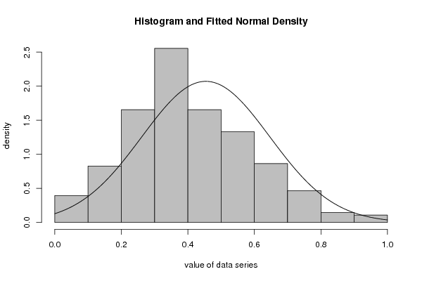
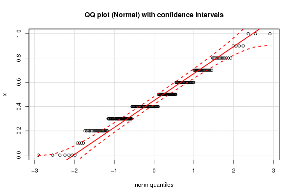
Title produced by software

ML Fitting and QQ Plot- Normal Distribution

Date of computation

Sun, 22 Jan 2017 12:09:04 +0100

Cite this page as follows

Statistical Computations at FreeStatistics.org, Office for Research Development and Education, URL https://freestatistics.org/blog/index.php?v=date/2017/Jan/22/t14850833833ck6f4veyg6y0qm.htm/, Retrieved Mon, 13 May 2024 22:51:59 +0000

Statistical Computations at FreeStatistics.org, Office for Research Development and Education, URL https://freestatistics.org/blog/index.php?pk=303348, Retrieved Mon, 13 May 2024 22:51:59 +0000

QR Codes:

Paste this QR Code to cite your computation.

Original text written by user:

IsPrivate?

No (this computation is public)

User-defined keywords

Estimated Impact

Family? (F = Feedback message, R = changed R code, M = changed R Module, P = changed Parameters, D = changed Data)

-       [ML Fitting and QQ Plot- Normal Distribution] [normal qq plot rf...] [2017-01-22 11:09:04] [d92250bd36540c2281a4ec15b45df1dd] [Current]

Feedback Forum

Post a new message

Dataseries X:

Download CSV

Histogram

Boxplots

0.5
0.5
0.4
0.5
0.7
0.3
0.4
0.4
0.7
0.6
0.6
0.2
0.4
0.4
0.5
0.3
0.4
0.7
0.5
0.2
0.3
0.6
0.6
0.2
0.7
0.2
1
0.4
0.4
0.2
0.4
0.4
0.7
0.2
0.6
0.3
0.3
0.2
0.5
0.7
0.6
0.4
0.6
0.4
0.3
0.5
0.2
0.3
0.5
0.7
0.4
0.3
0.2
0.5
0.4
0.6
0.4
0.4
0.2
0.9
0.8
0.8
0.3
0.2
0.4
0.2
0.2
0.1
0.4
0.5
0.8
0.4
0.6
0.5
0.3
0.4
0.6
0.4
0.3
0.8
0.6
0.3
0.5
0.4
0.3
0.7
0.2
0.4
0.6
0.6
0.6
0.4
0.6
0.5
0.5
0.6
0.8
0.5
0.6
0.4
0.3
0.3
0.2
0.4
0.5
0.3
0.4
0.5
0.3
0.5
0.4
0.4
0.6
0.3
0.4
0.3
1
0.4
0.8
0.3
0.5
0.4
0.3
0.5
0.3
0.3
0.4
0.3
0.6
0.6
0.4
0.4
0.4
0.3
0.2
0.5
0.4
0.4
0.4
0.3
0.4
0.2
0
0.4
0.6
0.4
0.4
0.4
0.2
0.4
0.3
0.6
0.6
0.4
0.5
0.4
0.6
0.6
0.9
0.4
0.8
0.5
0.4
0.4
0.7
0.4
0.8
0.4
0.3
0.5
0.8
0.4
1
0.5
0.5
0.3
0.3
0.3
0.4
0.5
0.5
0.4
0.7
0.5
0.4
0.7
0.7
0.7
0.7
0.7
0.7
0.1
0.2
0.3
0.6
0.8
0.8
0
0.3
0.6
0.5
0.7
0.3
0.3
0.4
0.4
0.1
0.5
0
0.4
0.6
0.4
0.1
0.3
0.7
0.3
0.5
0.3
0.6
0.9
0.4
0.3
0.9
0.5
0.3
0.6
0.2
0.4
0.5
0.4
0
0.2
0.5
0.3
0
0.5
0.6
0.3
0
0.3
0.5
0.4
0.5
0.7
0.8
0.6
0.4
0.5
0.5
0.3
0.6
0.3
0.6
0.3
0.7
0.7
0.6
0.5
0.5
0.4
0.4
0.7
0.2
0.5
0.4
0.2
0.5
0.4
0.7
0.6
0.4
0.5
0
0.7
0.4
0.5
0.6
0.8

Summary of computational transaction
Raw Input	view raw input (R code)
Raw Output	view raw output of R engine
Computing time	4 seconds
R Server	Big Analytics Cloud Computing Center

\begin{tabular}{lllllllll}
\hline
Summary of computational transaction \tabularnewline
Raw Input view raw input (R code)  \tabularnewline
Raw Outputview raw output of R engine  \tabularnewline
Computing time4 seconds \tabularnewline
R ServerBig Analytics Cloud Computing Center \tabularnewline
\hline
\end{tabular}
%Source: https://freestatistics.org/blog/index.php?pk=303348&T=0

[TABLE]
[ROW]

Summary of computational transaction[/C][/ROW] [ROW]

Raw Input[/C]

view raw input (R code) [/C][/ROW] [ROW]

Raw Output[/C]

view raw output of R engine [/C][/ROW] [ROW]

Computing time[/C]

4 seconds[/C][/ROW] [ROW]

R Server[/C]

Big Analytics Cloud Computing Center[/C][/ROW] [/TABLE] Source: https://freestatistics.org/blog/index.php?pk=303348&T=0

Globally Unique Identifier (entire table): ba.freestatistics.org/blog/index.php?pk=303348&T=0

As an alternative you can also use a QR Code:

The GUIDs for individual cells are displayed in the table below:

Summary of computational transaction
Raw Input	view raw input (R code)
Raw Output	view raw output of R engine
Computing time	4 seconds
R Server	Big Analytics Cloud Computing Center

Parameter	Estimated Value	Standard Deviation
mean	0.453956834532374	0.0115504305577424
standard deviation	0.192584163438342	0.00816738777300399

\begin{tabular}{lllllllll}
\hline
Parameter & Estimated Value & Standard Deviation \tabularnewline
mean & 0.453956834532374 & 0.0115504305577424 \tabularnewline
standard deviation & 0.192584163438342 & 0.00816738777300399 \tabularnewline
\hline
\end{tabular}
%Source: https://freestatistics.org/blog/index.php?pk=303348&T=1

[TABLE]
[ROW][C]Parameter[/C][C]Estimated Value[/C][C]Standard Deviation[/C][/ROW]
[ROW][C]mean[/C][C]0.453956834532374[/C][C]0.0115504305577424[/C][/ROW]
[ROW][C]standard deviation[/C][C]0.192584163438342[/C][C]0.00816738777300399[/C][/ROW]
[/TABLE]
Source: https://freestatistics.org/blog/index.php?pk=303348&T=1

Globally Unique Identifier (entire table): ba.freestatistics.org/blog/index.php?pk=303348&T=1

As an alternative you can also use a QR Code:

The GUIDs for individual cells are displayed in the table below:

Parameter	Estimated Value	Standard Deviation
mean	0.453956834532374	0.0115504305577424
standard deviation	0.192584163438342	0.00816738777300399

Figure 1

PNG link

Postscript link

PDF link

Figure 2

PNG link

Postscript link

PDF link

Parameters (Session):

par1 = 0.01 ; par2 = 0.99 ; par3 = 0.01 ;

Parameters (R input):

par1 = 8 ; par2 = 0 ;

R code (references can be found in the software module):

library(MASS)
library(car)
par1 <- as.numeric(par1)
if (par2 == '0') par2 = 'Sturges' else par2 <- as.numeric(par2)
x <- as.ts(x) #otherwise the fitdistr function does not work properly
r <- fitdistr(x,'normal')
print(r)
bitmap(file='test1.png')
myhist<-hist(x,col=par1,breaks=par2,main=main,ylab=ylab,xlab=xlab,freq=F)
curve(1/(r$estimate[2]*sqrt(2*pi))*exp(-1/2*((x-r$estimate[1])/r$estimate[2])^2),min(x),max(x),add=T)
dev.off()
bitmap(file='test3.png')
qqPlot(x,dist='norm',main='QQ plot (Normal) with confidence intervals')
grid()
dev.off()
load(file='createtable')
a<-table.start()
a<-table.row.start(a)
a<-table.element(a,'Parameter',1,TRUE)
a<-table.element(a,'Estimated Value',1,TRUE)
a<-table.element(a,'Standard Deviation',1,TRUE)
a<-table.row.end(a)
a<-table.row.start(a)
a<-table.element(a,'mean',header=TRUE)
a<-table.element(a,r$estimate[1])
a<-table.element(a,r$sd[1])
a<-table.row.end(a)
a<-table.row.start(a)
a<-table.element(a,'standard deviation',header=TRUE)
a<-table.element(a,r$estimate[2])
a<-table.element(a,r$sd[2])
a<-table.row.end(a)
a<-table.end(a)
table.save(a,file='mytable.tab')

Free Statistics

Description of Statistical Computation

Tree of Dependent Computations

Dataset

Tables (Output of Computation)

Figures (Output of Computation)

Input Parameters & R Code