Free Statistics

of Irreproducible Research!

Author's title

Author*Unverified author*
R Software Modulerwasp_decompose.wasp
Title produced by softwareClassical Decomposition
Date of computationWed, 04 Jan 2017 00:08:15 +0000
Cite this page as followsStatistical Computations at FreeStatistics.org, Office for Research Development and Education, URL https://freestatistics.org/blog/index.php?v=date/2017/Jan/04/t1483488524bzhwi32mnvtfgkp.htm/, Retrieved Tue, 14 May 2024 14:10:05 +0200
Statistical Computations at FreeStatistics.org, Office for Research Development and Education, URL https://freestatistics.org/blog/index.php?pk=, Retrieved Tue, 14 May 2024 14:10:05 +0200
QR Codes:

Original text written by user:
IsPrivate?No (this computation is public)
User-defined keywords
Estimated Impact0
Dataseries X:
1.336
1.3649
1.3999
1.4442
1.4349
1.4388
1.4264
1.4343
1.377
1.3706
1.3556
1.3179
1.2905
1.3224
1.3201
1.3162
1.2789
1.2526
1.2288
1.24
1.2856
1.2974
1.2828
1.3119
1.3288
1.3359
1.2964
1.3026
1.2982
1.3189
1.308
1.331
1.3348
1.3635
1.3493
1.3704
1.361
1.3658
1.3823
1.3812
1.3732
1.3592
1.3539
1.3316
1.2901
1.2673
1.2472
1.2331
1.1621
1.135
1.0838
1.0779
1.115
1.1213
1.0996
1.1139
1.1221
1.1235
1.0736
1.0877


Summary of computational transaction
Raw Inputview raw input (R code)
Raw Outputview raw output of R engine
Computing time1 seconds
R Server'Gwilym Jenkins' @ jenkins.wessa.net

\begin{tabular}{lllllllll}
\hline
Summary of computational transaction \tabularnewline
Raw Input & view raw input (R code)  \tabularnewline
Raw Output & view raw output of R engine  \tabularnewline
Computing time & 1 seconds \tabularnewline
R Server & 'Gwilym Jenkins' @ jenkins.wessa.net \tabularnewline
\hline
\end{tabular}
%Source: https://freestatistics.org/blog/index.php?pk=&T=0

[TABLE]
[ROW][C]Summary of computational transaction[/C][/ROW]
[ROW][C]Raw Input[/C][C]view raw input (R code) [/C][/ROW]
[ROW][C]Raw Output[/C][C]view raw output of R engine [/C][/ROW]
[ROW][C]Computing time[/C][C]1 seconds[/C][/ROW]
[ROW][C]R Server[/C][C]'Gwilym Jenkins' @ jenkins.wessa.net[/C][/ROW]
[/TABLE]
Source: https://freestatistics.org/blog/index.php?pk=&T=0

Globally Unique Identifier (entire table): ba.freestatistics.org/blog/index.php?pk=&T=0

As an alternative you can also use a QR Code:  

The GUIDs for individual cells are displayed in the table below:

Summary of computational transaction
Raw Inputview raw input (R code)
Raw Outputview raw output of R engine
Computing time1 seconds
R Server'Gwilym Jenkins' @ jenkins.wessa.net


Classical Decomposition by Moving Averages
tObservationsFitTrendSeasonalRandom
11.336NANA-0.0079592NA
21.3649NANA0.00295747NA
31.3999NANA-0.0101748NA
41.4442NANA-0.00612066NA
51.4349NANA-0.0037592NA
61.4388NANA-0.00174878NA
71.42641.388031.38981-0.001785240.0383727
81.43431.393521.386150.007371010.0407832
91.3771.381761.381050.000708507-0.00475851
101.37061.383031.372390.0106418-0.0124335
111.35561.362371.360560.00181476-0.00677309
121.31791.354351.34630.00805434-0.0364543
131.29051.322351.33031-0.0079592-0.0318491
141.32241.316941.313980.002957470.00546337
151.32011.29191.30207-0.01017480.0281998
161.31621.28911.29522-0.006120660.027104
171.27891.285371.28913-0.0037592-0.00647413
181.25261.28411.28585-0.00174878-0.0315012
191.22881.285411.2872-0.00178524-0.0566106
201.241.296731.289350.00737101-0.0567252
211.28561.289641.288930.000708507-0.00403767
221.29741.298021.287380.0106418-0.00061684
231.28281.289431.287610.00181476-0.00662726
241.31191.299231.291180.008054340.0126665
251.32881.289281.29724-0.00795920.0395175
261.33591.307291.304330.002957470.0286092
271.29641.31.31018-0.0101748-0.00360017
281.30261.308861.31498-0.00612066-0.00625851
291.29821.316741.3205-0.0037592-0.018545
301.31891.323961.32571-0.00174878-0.00506372
311.3081.327711.32949-0.00178524-0.0197064
321.3311.339451.332080.00737101-0.00845017
331.33481.337611.33690.000708507-0.00281267
341.36351.35441.343760.01064180.00909983
351.34931.351971.350160.00181476-0.00267309
361.37041.363021.354960.008054340.00738316
371.3611.350591.35855-0.00795920.010405
381.36581.363451.360490.002957470.00235087
391.38231.348481.35865-0.01017480.0338207
401.38121.346661.35278-0.006120660.0345373
411.37321.340761.34452-0.00375920.0324384
421.35921.33281.33455-0.001748780.026403
431.35391.318751.32054-0.001785240.0351477
441.33161.311.302630.007371010.0215957
451.29011.281291.280580.0007085070.00881233
461.26731.266151.25550.01064180.00115399
471.24721.233921.232110.001814760.0132769
481.23311.219491.211440.008054340.0136082
491.16211.182971.19093-0.0079592-0.02087
501.1351.174221.171260.00295747-0.03922
511.08381.145021.15519-0.0101748-0.0612168
521.07791.136081.1422-0.00612066-0.0581793
531.1151.125221.12898-0.0037592-0.0102158
541.12131.113931.11568-0.001748780.00736545
551.0996NANA-0.00178524NA
561.1139NANA0.00737101NA
571.1221NANA0.000708507NA
581.1235NANA0.0106418NA
591.0736NANA0.00181476NA
601.0877NANA0.00805434NA

\begin{tabular}{lllllllll}
\hline
Classical Decomposition by Moving Averages \tabularnewline
t & Observations & Fit & Trend & Seasonal & Random \tabularnewline
1 & 1.336 & NA & NA & -0.0079592 & NA \tabularnewline
2 & 1.3649 & NA & NA & 0.00295747 & NA \tabularnewline
3 & 1.3999 & NA & NA & -0.0101748 & NA \tabularnewline
4 & 1.4442 & NA & NA & -0.00612066 & NA \tabularnewline
5 & 1.4349 & NA & NA & -0.0037592 & NA \tabularnewline
6 & 1.4388 & NA & NA & -0.00174878 & NA \tabularnewline
7 & 1.4264 & 1.38803 & 1.38981 & -0.00178524 & 0.0383727 \tabularnewline
8 & 1.4343 & 1.39352 & 1.38615 & 0.00737101 & 0.0407832 \tabularnewline
9 & 1.377 & 1.38176 & 1.38105 & 0.000708507 & -0.00475851 \tabularnewline
10 & 1.3706 & 1.38303 & 1.37239 & 0.0106418 & -0.0124335 \tabularnewline
11 & 1.3556 & 1.36237 & 1.36056 & 0.00181476 & -0.00677309 \tabularnewline
12 & 1.3179 & 1.35435 & 1.3463 & 0.00805434 & -0.0364543 \tabularnewline
13 & 1.2905 & 1.32235 & 1.33031 & -0.0079592 & -0.0318491 \tabularnewline
14 & 1.3224 & 1.31694 & 1.31398 & 0.00295747 & 0.00546337 \tabularnewline
15 & 1.3201 & 1.2919 & 1.30207 & -0.0101748 & 0.0281998 \tabularnewline
16 & 1.3162 & 1.2891 & 1.29522 & -0.00612066 & 0.027104 \tabularnewline
17 & 1.2789 & 1.28537 & 1.28913 & -0.0037592 & -0.00647413 \tabularnewline
18 & 1.2526 & 1.2841 & 1.28585 & -0.00174878 & -0.0315012 \tabularnewline
19 & 1.2288 & 1.28541 & 1.2872 & -0.00178524 & -0.0566106 \tabularnewline
20 & 1.24 & 1.29673 & 1.28935 & 0.00737101 & -0.0567252 \tabularnewline
21 & 1.2856 & 1.28964 & 1.28893 & 0.000708507 & -0.00403767 \tabularnewline
22 & 1.2974 & 1.29802 & 1.28738 & 0.0106418 & -0.00061684 \tabularnewline
23 & 1.2828 & 1.28943 & 1.28761 & 0.00181476 & -0.00662726 \tabularnewline
24 & 1.3119 & 1.29923 & 1.29118 & 0.00805434 & 0.0126665 \tabularnewline
25 & 1.3288 & 1.28928 & 1.29724 & -0.0079592 & 0.0395175 \tabularnewline
26 & 1.3359 & 1.30729 & 1.30433 & 0.00295747 & 0.0286092 \tabularnewline
27 & 1.2964 & 1.3 & 1.31018 & -0.0101748 & -0.00360017 \tabularnewline
28 & 1.3026 & 1.30886 & 1.31498 & -0.00612066 & -0.00625851 \tabularnewline
29 & 1.2982 & 1.31674 & 1.3205 & -0.0037592 & -0.018545 \tabularnewline
30 & 1.3189 & 1.32396 & 1.32571 & -0.00174878 & -0.00506372 \tabularnewline
31 & 1.308 & 1.32771 & 1.32949 & -0.00178524 & -0.0197064 \tabularnewline
32 & 1.331 & 1.33945 & 1.33208 & 0.00737101 & -0.00845017 \tabularnewline
33 & 1.3348 & 1.33761 & 1.3369 & 0.000708507 & -0.00281267 \tabularnewline
34 & 1.3635 & 1.3544 & 1.34376 & 0.0106418 & 0.00909983 \tabularnewline
35 & 1.3493 & 1.35197 & 1.35016 & 0.00181476 & -0.00267309 \tabularnewline
36 & 1.3704 & 1.36302 & 1.35496 & 0.00805434 & 0.00738316 \tabularnewline
37 & 1.361 & 1.35059 & 1.35855 & -0.0079592 & 0.010405 \tabularnewline
38 & 1.3658 & 1.36345 & 1.36049 & 0.00295747 & 0.00235087 \tabularnewline
39 & 1.3823 & 1.34848 & 1.35865 & -0.0101748 & 0.0338207 \tabularnewline
40 & 1.3812 & 1.34666 & 1.35278 & -0.00612066 & 0.0345373 \tabularnewline
41 & 1.3732 & 1.34076 & 1.34452 & -0.0037592 & 0.0324384 \tabularnewline
42 & 1.3592 & 1.3328 & 1.33455 & -0.00174878 & 0.026403 \tabularnewline
43 & 1.3539 & 1.31875 & 1.32054 & -0.00178524 & 0.0351477 \tabularnewline
44 & 1.3316 & 1.31 & 1.30263 & 0.00737101 & 0.0215957 \tabularnewline
45 & 1.2901 & 1.28129 & 1.28058 & 0.000708507 & 0.00881233 \tabularnewline
46 & 1.2673 & 1.26615 & 1.2555 & 0.0106418 & 0.00115399 \tabularnewline
47 & 1.2472 & 1.23392 & 1.23211 & 0.00181476 & 0.0132769 \tabularnewline
48 & 1.2331 & 1.21949 & 1.21144 & 0.00805434 & 0.0136082 \tabularnewline
49 & 1.1621 & 1.18297 & 1.19093 & -0.0079592 & -0.02087 \tabularnewline
50 & 1.135 & 1.17422 & 1.17126 & 0.00295747 & -0.03922 \tabularnewline
51 & 1.0838 & 1.14502 & 1.15519 & -0.0101748 & -0.0612168 \tabularnewline
52 & 1.0779 & 1.13608 & 1.1422 & -0.00612066 & -0.0581793 \tabularnewline
53 & 1.115 & 1.12522 & 1.12898 & -0.0037592 & -0.0102158 \tabularnewline
54 & 1.1213 & 1.11393 & 1.11568 & -0.00174878 & 0.00736545 \tabularnewline
55 & 1.0996 & NA & NA & -0.00178524 & NA \tabularnewline
56 & 1.1139 & NA & NA & 0.00737101 & NA \tabularnewline
57 & 1.1221 & NA & NA & 0.000708507 & NA \tabularnewline
58 & 1.1235 & NA & NA & 0.0106418 & NA \tabularnewline
59 & 1.0736 & NA & NA & 0.00181476 & NA \tabularnewline
60 & 1.0877 & NA & NA & 0.00805434 & NA \tabularnewline
\hline
\end{tabular}
%Source: https://freestatistics.org/blog/index.php?pk=&T=1

[TABLE]
[ROW][C]Classical Decomposition by Moving Averages[/C][/ROW]
[ROW][C]t[/C][C]Observations[/C][C]Fit[/C][C]Trend[/C][C]Seasonal[/C][C]Random[/C][/ROW]
[ROW][C]1[/C][C]1.336[/C][C]NA[/C][C]NA[/C][C]-0.0079592[/C][C]NA[/C][/ROW]
[ROW][C]2[/C][C]1.3649[/C][C]NA[/C][C]NA[/C][C]0.00295747[/C][C]NA[/C][/ROW]
[ROW][C]3[/C][C]1.3999[/C][C]NA[/C][C]NA[/C][C]-0.0101748[/C][C]NA[/C][/ROW]
[ROW][C]4[/C][C]1.4442[/C][C]NA[/C][C]NA[/C][C]-0.00612066[/C][C]NA[/C][/ROW]
[ROW][C]5[/C][C]1.4349[/C][C]NA[/C][C]NA[/C][C]-0.0037592[/C][C]NA[/C][/ROW]
[ROW][C]6[/C][C]1.4388[/C][C]NA[/C][C]NA[/C][C]-0.00174878[/C][C]NA[/C][/ROW]
[ROW][C]7[/C][C]1.4264[/C][C]1.38803[/C][C]1.38981[/C][C]-0.00178524[/C][C]0.0383727[/C][/ROW]
[ROW][C]8[/C][C]1.4343[/C][C]1.39352[/C][C]1.38615[/C][C]0.00737101[/C][C]0.0407832[/C][/ROW]
[ROW][C]9[/C][C]1.377[/C][C]1.38176[/C][C]1.38105[/C][C]0.000708507[/C][C]-0.00475851[/C][/ROW]
[ROW][C]10[/C][C]1.3706[/C][C]1.38303[/C][C]1.37239[/C][C]0.0106418[/C][C]-0.0124335[/C][/ROW]
[ROW][C]11[/C][C]1.3556[/C][C]1.36237[/C][C]1.36056[/C][C]0.00181476[/C][C]-0.00677309[/C][/ROW]
[ROW][C]12[/C][C]1.3179[/C][C]1.35435[/C][C]1.3463[/C][C]0.00805434[/C][C]-0.0364543[/C][/ROW]
[ROW][C]13[/C][C]1.2905[/C][C]1.32235[/C][C]1.33031[/C][C]-0.0079592[/C][C]-0.0318491[/C][/ROW]
[ROW][C]14[/C][C]1.3224[/C][C]1.31694[/C][C]1.31398[/C][C]0.00295747[/C][C]0.00546337[/C][/ROW]
[ROW][C]15[/C][C]1.3201[/C][C]1.2919[/C][C]1.30207[/C][C]-0.0101748[/C][C]0.0281998[/C][/ROW]
[ROW][C]16[/C][C]1.3162[/C][C]1.2891[/C][C]1.29522[/C][C]-0.00612066[/C][C]0.027104[/C][/ROW]
[ROW][C]17[/C][C]1.2789[/C][C]1.28537[/C][C]1.28913[/C][C]-0.0037592[/C][C]-0.00647413[/C][/ROW]
[ROW][C]18[/C][C]1.2526[/C][C]1.2841[/C][C]1.28585[/C][C]-0.00174878[/C][C]-0.0315012[/C][/ROW]
[ROW][C]19[/C][C]1.2288[/C][C]1.28541[/C][C]1.2872[/C][C]-0.00178524[/C][C]-0.0566106[/C][/ROW]
[ROW][C]20[/C][C]1.24[/C][C]1.29673[/C][C]1.28935[/C][C]0.00737101[/C][C]-0.0567252[/C][/ROW]
[ROW][C]21[/C][C]1.2856[/C][C]1.28964[/C][C]1.28893[/C][C]0.000708507[/C][C]-0.00403767[/C][/ROW]
[ROW][C]22[/C][C]1.2974[/C][C]1.29802[/C][C]1.28738[/C][C]0.0106418[/C][C]-0.00061684[/C][/ROW]
[ROW][C]23[/C][C]1.2828[/C][C]1.28943[/C][C]1.28761[/C][C]0.00181476[/C][C]-0.00662726[/C][/ROW]
[ROW][C]24[/C][C]1.3119[/C][C]1.29923[/C][C]1.29118[/C][C]0.00805434[/C][C]0.0126665[/C][/ROW]
[ROW][C]25[/C][C]1.3288[/C][C]1.28928[/C][C]1.29724[/C][C]-0.0079592[/C][C]0.0395175[/C][/ROW]
[ROW][C]26[/C][C]1.3359[/C][C]1.30729[/C][C]1.30433[/C][C]0.00295747[/C][C]0.0286092[/C][/ROW]
[ROW][C]27[/C][C]1.2964[/C][C]1.3[/C][C]1.31018[/C][C]-0.0101748[/C][C]-0.00360017[/C][/ROW]
[ROW][C]28[/C][C]1.3026[/C][C]1.30886[/C][C]1.31498[/C][C]-0.00612066[/C][C]-0.00625851[/C][/ROW]
[ROW][C]29[/C][C]1.2982[/C][C]1.31674[/C][C]1.3205[/C][C]-0.0037592[/C][C]-0.018545[/C][/ROW]
[ROW][C]30[/C][C]1.3189[/C][C]1.32396[/C][C]1.32571[/C][C]-0.00174878[/C][C]-0.00506372[/C][/ROW]
[ROW][C]31[/C][C]1.308[/C][C]1.32771[/C][C]1.32949[/C][C]-0.00178524[/C][C]-0.0197064[/C][/ROW]
[ROW][C]32[/C][C]1.331[/C][C]1.33945[/C][C]1.33208[/C][C]0.00737101[/C][C]-0.00845017[/C][/ROW]
[ROW][C]33[/C][C]1.3348[/C][C]1.33761[/C][C]1.3369[/C][C]0.000708507[/C][C]-0.00281267[/C][/ROW]
[ROW][C]34[/C][C]1.3635[/C][C]1.3544[/C][C]1.34376[/C][C]0.0106418[/C][C]0.00909983[/C][/ROW]
[ROW][C]35[/C][C]1.3493[/C][C]1.35197[/C][C]1.35016[/C][C]0.00181476[/C][C]-0.00267309[/C][/ROW]
[ROW][C]36[/C][C]1.3704[/C][C]1.36302[/C][C]1.35496[/C][C]0.00805434[/C][C]0.00738316[/C][/ROW]
[ROW][C]37[/C][C]1.361[/C][C]1.35059[/C][C]1.35855[/C][C]-0.0079592[/C][C]0.010405[/C][/ROW]
[ROW][C]38[/C][C]1.3658[/C][C]1.36345[/C][C]1.36049[/C][C]0.00295747[/C][C]0.00235087[/C][/ROW]
[ROW][C]39[/C][C]1.3823[/C][C]1.34848[/C][C]1.35865[/C][C]-0.0101748[/C][C]0.0338207[/C][/ROW]
[ROW][C]40[/C][C]1.3812[/C][C]1.34666[/C][C]1.35278[/C][C]-0.00612066[/C][C]0.0345373[/C][/ROW]
[ROW][C]41[/C][C]1.3732[/C][C]1.34076[/C][C]1.34452[/C][C]-0.0037592[/C][C]0.0324384[/C][/ROW]
[ROW][C]42[/C][C]1.3592[/C][C]1.3328[/C][C]1.33455[/C][C]-0.00174878[/C][C]0.026403[/C][/ROW]
[ROW][C]43[/C][C]1.3539[/C][C]1.31875[/C][C]1.32054[/C][C]-0.00178524[/C][C]0.0351477[/C][/ROW]
[ROW][C]44[/C][C]1.3316[/C][C]1.31[/C][C]1.30263[/C][C]0.00737101[/C][C]0.0215957[/C][/ROW]
[ROW][C]45[/C][C]1.2901[/C][C]1.28129[/C][C]1.28058[/C][C]0.000708507[/C][C]0.00881233[/C][/ROW]
[ROW][C]46[/C][C]1.2673[/C][C]1.26615[/C][C]1.2555[/C][C]0.0106418[/C][C]0.00115399[/C][/ROW]
[ROW][C]47[/C][C]1.2472[/C][C]1.23392[/C][C]1.23211[/C][C]0.00181476[/C][C]0.0132769[/C][/ROW]
[ROW][C]48[/C][C]1.2331[/C][C]1.21949[/C][C]1.21144[/C][C]0.00805434[/C][C]0.0136082[/C][/ROW]
[ROW][C]49[/C][C]1.1621[/C][C]1.18297[/C][C]1.19093[/C][C]-0.0079592[/C][C]-0.02087[/C][/ROW]
[ROW][C]50[/C][C]1.135[/C][C]1.17422[/C][C]1.17126[/C][C]0.00295747[/C][C]-0.03922[/C][/ROW]
[ROW][C]51[/C][C]1.0838[/C][C]1.14502[/C][C]1.15519[/C][C]-0.0101748[/C][C]-0.0612168[/C][/ROW]
[ROW][C]52[/C][C]1.0779[/C][C]1.13608[/C][C]1.1422[/C][C]-0.00612066[/C][C]-0.0581793[/C][/ROW]
[ROW][C]53[/C][C]1.115[/C][C]1.12522[/C][C]1.12898[/C][C]-0.0037592[/C][C]-0.0102158[/C][/ROW]
[ROW][C]54[/C][C]1.1213[/C][C]1.11393[/C][C]1.11568[/C][C]-0.00174878[/C][C]0.00736545[/C][/ROW]
[ROW][C]55[/C][C]1.0996[/C][C]NA[/C][C]NA[/C][C]-0.00178524[/C][C]NA[/C][/ROW]
[ROW][C]56[/C][C]1.1139[/C][C]NA[/C][C]NA[/C][C]0.00737101[/C][C]NA[/C][/ROW]
[ROW][C]57[/C][C]1.1221[/C][C]NA[/C][C]NA[/C][C]0.000708507[/C][C]NA[/C][/ROW]
[ROW][C]58[/C][C]1.1235[/C][C]NA[/C][C]NA[/C][C]0.0106418[/C][C]NA[/C][/ROW]
[ROW][C]59[/C][C]1.0736[/C][C]NA[/C][C]NA[/C][C]0.00181476[/C][C]NA[/C][/ROW]
[ROW][C]60[/C][C]1.0877[/C][C]NA[/C][C]NA[/C][C]0.00805434[/C][C]NA[/C][/ROW]
[/TABLE]
Source: https://freestatistics.org/blog/index.php?pk=&T=1

Globally Unique Identifier (entire table): ba.freestatistics.org/blog/index.php?pk=&T=1

As an alternative you can also use a QR Code:  

The GUIDs for individual cells are displayed in the table below:

Classical Decomposition by Moving Averages
tObservationsFitTrendSeasonalRandom
11.336NANA-0.0079592NA
21.3649NANA0.00295747NA
31.3999NANA-0.0101748NA
41.4442NANA-0.00612066NA
51.4349NANA-0.0037592NA
61.4388NANA-0.00174878NA
71.42641.388031.38981-0.001785240.0383727
81.43431.393521.386150.007371010.0407832
91.3771.381761.381050.000708507-0.00475851
101.37061.383031.372390.0106418-0.0124335
111.35561.362371.360560.00181476-0.00677309
121.31791.354351.34630.00805434-0.0364543
131.29051.322351.33031-0.0079592-0.0318491
141.32241.316941.313980.002957470.00546337
151.32011.29191.30207-0.01017480.0281998
161.31621.28911.29522-0.006120660.027104
171.27891.285371.28913-0.0037592-0.00647413
181.25261.28411.28585-0.00174878-0.0315012
191.22881.285411.2872-0.00178524-0.0566106
201.241.296731.289350.00737101-0.0567252
211.28561.289641.288930.000708507-0.00403767
221.29741.298021.287380.0106418-0.00061684
231.28281.289431.287610.00181476-0.00662726
241.31191.299231.291180.008054340.0126665
251.32881.289281.29724-0.00795920.0395175
261.33591.307291.304330.002957470.0286092
271.29641.31.31018-0.0101748-0.00360017
281.30261.308861.31498-0.00612066-0.00625851
291.29821.316741.3205-0.0037592-0.018545
301.31891.323961.32571-0.00174878-0.00506372
311.3081.327711.32949-0.00178524-0.0197064
321.3311.339451.332080.00737101-0.00845017
331.33481.337611.33690.000708507-0.00281267
341.36351.35441.343760.01064180.00909983
351.34931.351971.350160.00181476-0.00267309
361.37041.363021.354960.008054340.00738316
371.3611.350591.35855-0.00795920.010405
381.36581.363451.360490.002957470.00235087
391.38231.348481.35865-0.01017480.0338207
401.38121.346661.35278-0.006120660.0345373
411.37321.340761.34452-0.00375920.0324384
421.35921.33281.33455-0.001748780.026403
431.35391.318751.32054-0.001785240.0351477
441.33161.311.302630.007371010.0215957
451.29011.281291.280580.0007085070.00881233
461.26731.266151.25550.01064180.00115399
471.24721.233921.232110.001814760.0132769
481.23311.219491.211440.008054340.0136082
491.16211.182971.19093-0.0079592-0.02087
501.1351.174221.171260.00295747-0.03922
511.08381.145021.15519-0.0101748-0.0612168
521.07791.136081.1422-0.00612066-0.0581793
531.1151.125221.12898-0.0037592-0.0102158
541.12131.113931.11568-0.001748780.00736545
551.0996NANA-0.00178524NA
561.1139NANA0.00737101NA
571.1221NANA0.000708507NA
581.1235NANA0.0106418NA
591.0736NANA0.00181476NA
601.0877NANA0.00805434NA


Parameters (Session):
par1 = 0.01 ; par2 = 0.99 ; par3 = 0.01 ;
Parameters (R input):
par1 = additive ; par2 = 12 ;
R code (references can be found in the software module):
par2 <- as.numeric(par2)
x <- ts(x,freq=par2)
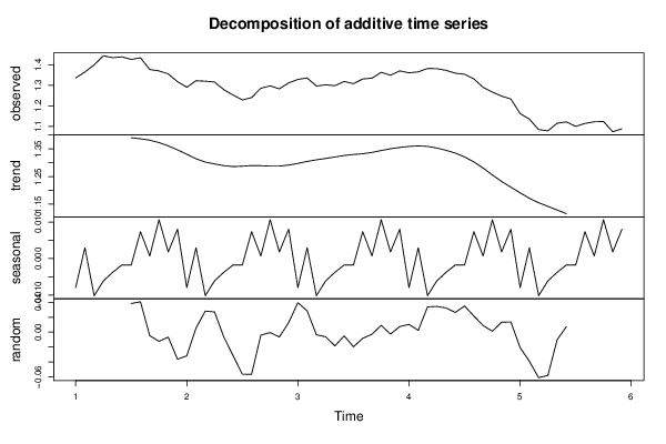
m <- decompose(x,type=par1)
m$figure
bitmap(file='test1.png')
plot(m)
dev.off()
mylagmax <- length(x)/2
bitmap(file='test2.png')
op <- par(mfrow = c(2,2))
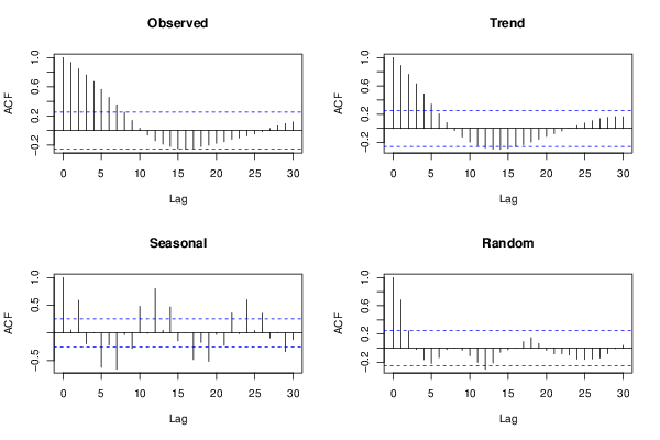
acf(as.numeric(x),lag.max = mylagmax,main='Observed')
acf(as.numeric(m$trend),na.action=na.pass,lag.max = mylagmax,main='Trend')
acf(as.numeric(m$seasonal),na.action=na.pass,lag.max = mylagmax,main='Seasonal')
acf(as.numeric(m$random),na.action=na.pass,lag.max = mylagmax,main='Random')
par(op)
dev.off()
bitmap(file='test3.png')
op <- par(mfrow = c(2,2))
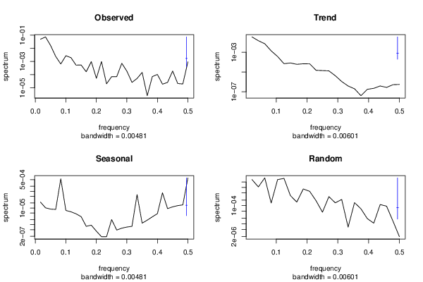
spectrum(as.numeric(x),main='Observed')
spectrum(as.numeric(m$trend[!is.na(m$trend)]),main='Trend')
spectrum(as.numeric(m$seasonal[!is.na(m$seasonal)]),main='Seasonal')
spectrum(as.numeric(m$random[!is.na(m$random)]),main='Random')
par(op)
dev.off()
bitmap(file='test4.png')
op <- par(mfrow = c(2,2))
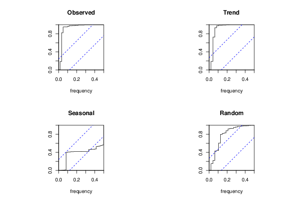
cpgram(as.numeric(x),main='Observed')
cpgram(as.numeric(m$trend[!is.na(m$trend)]),main='Trend')
cpgram(as.numeric(m$seasonal[!is.na(m$seasonal)]),main='Seasonal')
cpgram(as.numeric(m$random[!is.na(m$random)]),main='Random')
par(op)
dev.off()
load(file='createtable')
a<-table.start()
a<-table.row.start(a)
a<-table.element(a,'Classical Decomposition by Moving Averages',6,TRUE)
a<-table.row.end(a)
a<-table.row.start(a)
a<-table.element(a,'t',header=TRUE)
a<-table.element(a,'Observations',header=TRUE)
a<-table.element(a,'Fit',header=TRUE)
a<-table.element(a,'Trend',header=TRUE)
a<-table.element(a,'Seasonal',header=TRUE)
a<-table.element(a,'Random',header=TRUE)
a<-table.row.end(a)
for (i in 1:length(m$trend)) {
a<-table.row.start(a)
a<-table.element(a,i,header=TRUE)
a<-table.element(a,x[i])
if (par1 == 'additive') a<-table.element(a,signif(m$trend[i]+m$seasonal[i],6)) else a<-table.element(a,signif(m$trend[i]*m$seasonal[i],6))
a<-table.element(a,signif(m$trend[i],6))
a<-table.element(a,signif(m$seasonal[i],6))
a<-table.element(a,signif(m$random[i],6))
a<-table.row.end(a)
}
a<-table.end(a)
table.save(a,file='mytable.tab')