Free Statistics
of Irreproducible Research!
Description of Statistical Computation | |||||||||||||||||||||
|---|---|---|---|---|---|---|---|---|---|---|---|---|---|---|---|---|---|---|---|---|---|
| Author's title | |||||||||||||||||||||
| Author | *Unverified author* | ||||||||||||||||||||
| R Software Module | rwasp_meanplot.wasp | ||||||||||||||||||||
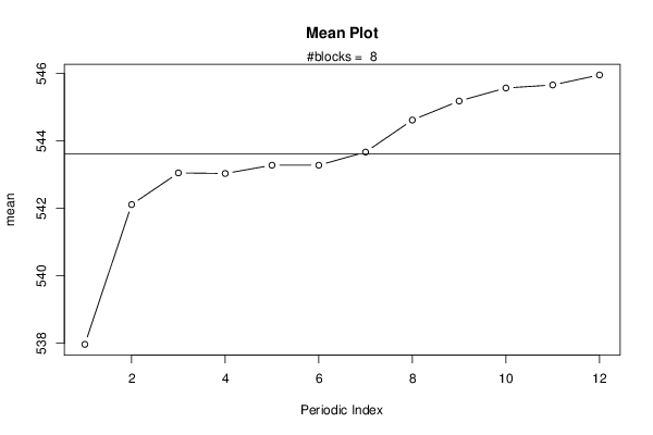
| Title produced by software | Mean Plot | ||||||||||||||||||||
| Date of computation | Tue, 26 May 2015 15:46:45 +0100 | ||||||||||||||||||||
| Cite this page as follows | Statistical Computations at FreeStatistics.org, Office for Research Development and Education, URL https://freestatistics.org/blog/index.php?v=date/2015/May/26/t1432651785hcts6i2mf0z5ruh.htm/, Retrieved Tue, 30 Apr 2024 18:58:57 +0000 | ||||||||||||||||||||
| Statistical Computations at FreeStatistics.org, Office for Research Development and Education, URL https://freestatistics.org/blog/index.php?pk=279393, Retrieved Tue, 30 Apr 2024 18:58:57 +0000 | |||||||||||||||||||||
| QR Codes: | |||||||||||||||||||||
|
| |||||||||||||||||||||
| Original text written by user: | |||||||||||||||||||||
| IsPrivate? | No (this computation is public) | ||||||||||||||||||||
| User-defined keywords | |||||||||||||||||||||
| Estimated Impact | 115 | ||||||||||||||||||||
Tree of Dependent Computations | |||||||||||||||||||||
| Family? (F = Feedback message, R = changed R code, M = changed R Module, P = changed Parameters, D = changed Data) | |||||||||||||||||||||
| - [Mean Plot] [Mean Plot luchtva...] [2015-02-26 15:46:06] [77cae2e8655af67d2d17f40c5b6aa8cb] - D [Mean Plot] [] [2015-05-26 14:46:45] [1689e0541609f8eb663ad6752b966f5b] [Current] | |||||||||||||||||||||
| Feedback Forum | |||||||||||||||||||||
Post a new message | |||||||||||||||||||||
Dataset | |||||||||||||||||||||
| Dataseries X: | |||||||||||||||||||||
498.10 498.76 498.88 498.88 498.88 498.88 499.48 501.21 502.05 502.05 502.05 504.10 506.81 516.88 520.43 520.68 520.68 520.68 521.03 521.25 521.25 521.25 521.65 521.65 522.77 518.72 519.27 519.38 521.29 521.29 521.29 523.47 523.86 524.14 524.14 524.14 534.60 534.99 535.39 535.39 535.39 535.39 535.39 535.64 536.08 537.80 537.80 537.80 537.85 544.39 545.15 544.65 544.65 544.65 545.73 548.94 550.94 551.22 551.22 551.22 553.12 565.37 566.73 566.73 566.78 566.78 566.78 566.78 566.93 566.93 566.93 566.93 574.38 574.40 574.40 574.40 574.40 574.40 574.50 574.50 574.67 574.66 574.66 574.94 576.10 583.38 584.15 584.15 584.15 584.15 585.14 585.14 585.67 586.49 586.81 586.85 | |||||||||||||||||||||
Tables (Output of Computation) | |||||||||||||||||||||
| |||||||||||||||||||||
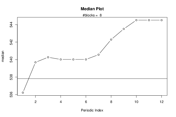
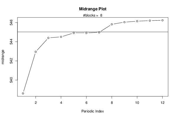
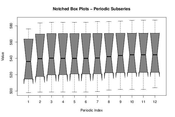
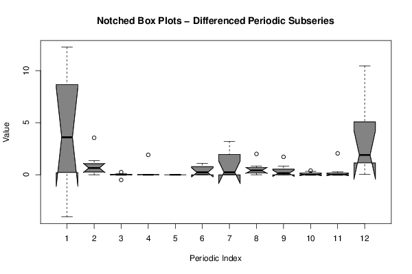
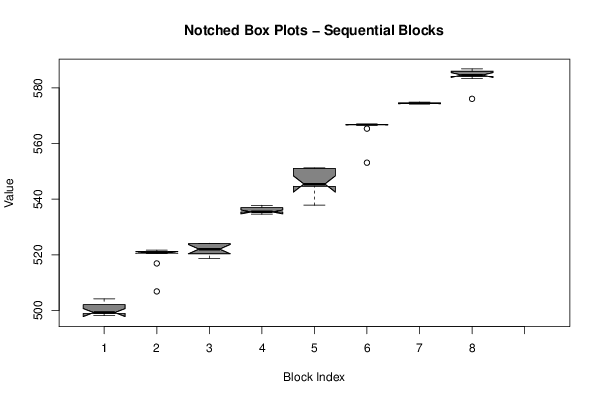
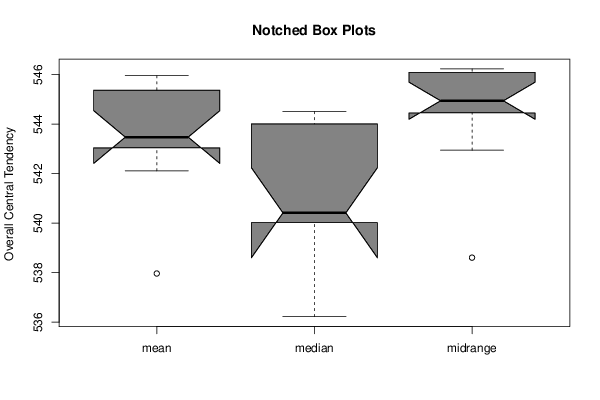
Figures (Output of Computation) | |||||||||||||||||||||
Input Parameters & R Code | |||||||||||||||||||||
| Parameters (Session): | |||||||||||||||||||||
| par1 = 12 ; | |||||||||||||||||||||
| Parameters (R input): | |||||||||||||||||||||
| par1 = 12 ; | |||||||||||||||||||||
| R code (references can be found in the software module): | |||||||||||||||||||||
par1 <- as.numeric(par1) | |||||||||||||||||||||