Free Statistics
of Irreproducible Research!
Description of Statistical Computation | |||||||||||||||||||||
|---|---|---|---|---|---|---|---|---|---|---|---|---|---|---|---|---|---|---|---|---|---|
| Author's title | |||||||||||||||||||||
| Author | *Unverified author* | ||||||||||||||||||||
| R Software Module | rwasp_meanplot.wasp | ||||||||||||||||||||
| Title produced by software | Mean Plot | ||||||||||||||||||||
| Date of computation | Tue, 26 May 2015 12:47:19 +0100 | ||||||||||||||||||||
| Cite this page as follows | Statistical Computations at FreeStatistics.org, Office for Research Development and Education, URL https://freestatistics.org/blog/index.php?v=date/2015/May/26/t14326408883e6bcp92ijnxi4o.htm/, Retrieved Tue, 30 Apr 2024 13:40:54 +0000 | ||||||||||||||||||||
| Statistical Computations at FreeStatistics.org, Office for Research Development and Education, URL https://freestatistics.org/blog/index.php?pk=279389, Retrieved Tue, 30 Apr 2024 13:40:54 +0000 | |||||||||||||||||||||
| QR Codes: | |||||||||||||||||||||
|
| |||||||||||||||||||||
| Original text written by user: | |||||||||||||||||||||
| IsPrivate? | No (this computation is public) | ||||||||||||||||||||
| User-defined keywords | |||||||||||||||||||||
| Estimated Impact | 112 | ||||||||||||||||||||
Tree of Dependent Computations | |||||||||||||||||||||
| Family? (F = Feedback message, R = changed R code, M = changed R Module, P = changed Parameters, D = changed Data) | |||||||||||||||||||||
| - [Mean Plot] [Mean Plot luchtva...] [2015-02-26 15:46:06] [77cae2e8655af67d2d17f40c5b6aa8cb] - [Mean Plot] [] [2015-05-26 11:47:19] [1689e0541609f8eb663ad6752b966f5b] [Current] | |||||||||||||||||||||
| Feedback Forum | |||||||||||||||||||||
Post a new message | |||||||||||||||||||||
Dataset | |||||||||||||||||||||
| Dataseries X: | |||||||||||||||||||||
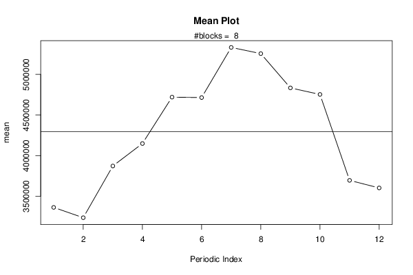
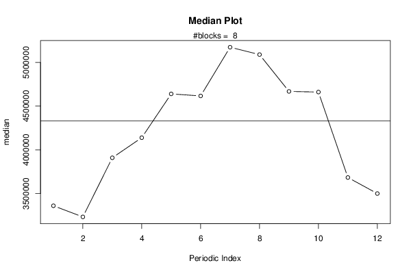
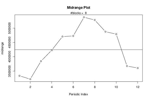
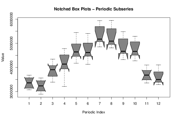
3167956,00 3001753,00 3571343,00 3990145,00 4472259,00 4487988,00 5021544,00 4877589,00 4563348,00 4452338,00 3535989,00 3454304,00 3331523,00 3213977,00 3896807,00 4121803,00 4566599,00 4529566,00 5172312,00 5121598,00 4713449,00 4656638,00 3647578,00 3545823,00 3388686,00 3348700,00 3973721,00 4156519,00 4713826,00 4704148,00 5175950,00 5025767,00 4600637,00 4560314,00 3443549,00 3333873,00 3072606,00 2891262,00 3390581,00 3888685,00 4173577,00 4130139,00 4851476,00 4811406,00 4322719,00 4274814,00 3355439,00 3293039,00 3114971,00 3049444,00 3697355,00 3213665,00 4447089,00 4442139,00 5119203,00 5058056,00 4623783,00 4666071,00 3719403,00 3440349,00 3466587,00 3251624,00 3921482,00 4466794,00 4916693,00 4939490,00 5627276,00 5540569,00 5128892,00 5024163,00 3807138,00 3777434,00 3675761,00 3552136,00 4177498,00 4568847,00 5027940,00 5078079,00 5759003,00 5671424,00 5239374,00 5100023,00 3944666,00 3858569,00 3670053,00 3563751,00 4341934,00 4779391,00 5440427,00 5404974,00 5934128,00 5942981,00 5477811,00 5288928,00 4099344,00 4103791,00 | |||||||||||||||||||||
Tables (Output of Computation) | |||||||||||||||||||||
| |||||||||||||||||||||
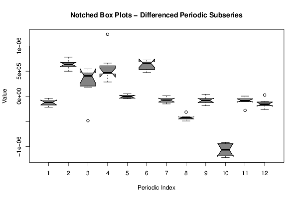
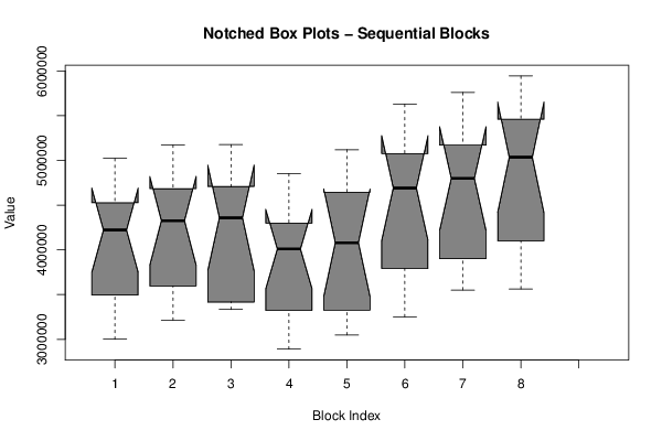
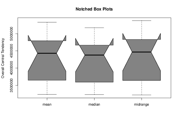
Figures (Output of Computation) | |||||||||||||||||||||
Input Parameters & R Code | |||||||||||||||||||||
| Parameters (Session): | |||||||||||||||||||||
| par1 = 12 ; | |||||||||||||||||||||
| Parameters (R input): | |||||||||||||||||||||
| par1 = 12 ; | |||||||||||||||||||||
| R code (references can be found in the software module): | |||||||||||||||||||||
par1 <- as.numeric(par1) | |||||||||||||||||||||