Free Statistics
of Irreproducible Research!
Description of Statistical Computation | |||||||||||||||||||||
|---|---|---|---|---|---|---|---|---|---|---|---|---|---|---|---|---|---|---|---|---|---|
| Author's title | |||||||||||||||||||||
| Author | *Unverified author* | ||||||||||||||||||||
| R Software Module | rwasp_meanplot.wasp | ||||||||||||||||||||
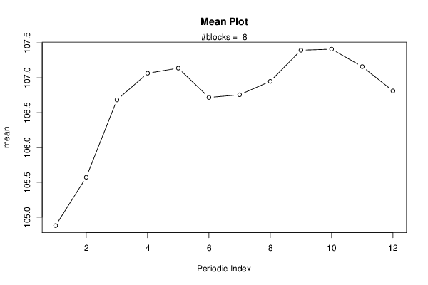
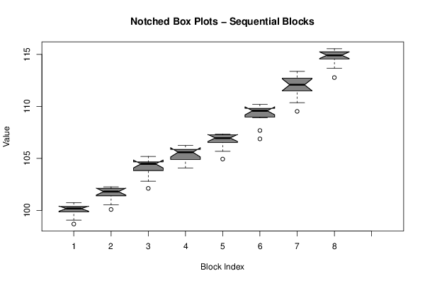
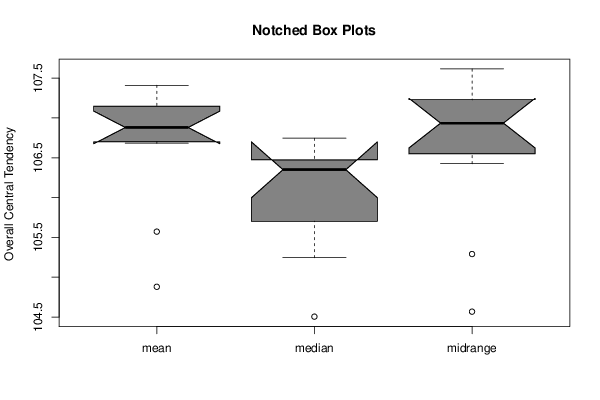
| Title produced by software | Mean Plot | ||||||||||||||||||||
| Date of computation | Wed, 20 May 2015 12:58:02 +0100 | ||||||||||||||||||||
| Cite this page as follows | Statistical Computations at FreeStatistics.org, Office for Research Development and Education, URL https://freestatistics.org/blog/index.php?v=date/2015/May/20/t1432123161cpwdt3aq4xg9ec0.htm/, Retrieved Mon, 29 Apr 2024 12:44:17 +0000 | ||||||||||||||||||||
| Statistical Computations at FreeStatistics.org, Office for Research Development and Education, URL https://freestatistics.org/blog/index.php?pk=279164, Retrieved Mon, 29 Apr 2024 12:44:17 +0000 | |||||||||||||||||||||
| QR Codes: | |||||||||||||||||||||
|
| |||||||||||||||||||||
| Original text written by user: | |||||||||||||||||||||
| IsPrivate? | No (this computation is public) | ||||||||||||||||||||
| User-defined keywords | |||||||||||||||||||||
| Estimated Impact | 131 | ||||||||||||||||||||
Tree of Dependent Computations | |||||||||||||||||||||
| Family? (F = Feedback message, R = changed R code, M = changed R Module, P = changed Parameters, D = changed Data) | |||||||||||||||||||||
| - [Mean Plot] [consumentenprijze...] [2015-05-20 11:58:02] [0793dda36b6d92f80d1980fc1d00d6bd] [Current] | |||||||||||||||||||||
| Feedback Forum | |||||||||||||||||||||
Post a new message | |||||||||||||||||||||
Dataset | |||||||||||||||||||||
| Dataseries X: | |||||||||||||||||||||
98,68 99,06 99,84 100,3 100,38 100,02 99,83 100,36 100,74 100,49 100,33 99,96 100,08 100,54 101,63 102,12 102,19 101,77 101,29 101,47 102,07 102,11 102,26 101,83 102,11 102,8 103,82 104,2 104,57 104,38 104,54 104,74 105,19 104,95 104,57 103,81 104,08 104,81 105,86 106,1 106,24 105,87 104,74 105,03 105,59 105,69 105,58 104,96 104,93 105,68 106,93 107,29 107,25 106,74 106,44 106,6 107,26 107,35 107,22 106,99 106,87 107,68 108,9 109,48 109,57 109,03 109,58 109,76 110,15 110,2 109,86 109,58 109,52 110,35 111,61 112,06 111,9 111,36 112,09 112,24 112,7 113,36 112,9 112,74 112,77 113,66 114,87 114,97 115 114,57 115,54 115,39 115,46 115,13 114,56 114,62 | |||||||||||||||||||||
Tables (Output of Computation) | |||||||||||||||||||||
| |||||||||||||||||||||
Figures (Output of Computation) | |||||||||||||||||||||
Input Parameters & R Code | |||||||||||||||||||||
| Parameters (Session): | |||||||||||||||||||||
| par1 = 4 ; par2 = no ; par3 = 512 ; | |||||||||||||||||||||
| Parameters (R input): | |||||||||||||||||||||
| par1 = 12 ; | |||||||||||||||||||||
| R code (references can be found in the software module): | |||||||||||||||||||||
par1 <- as.numeric(par1) | |||||||||||||||||||||