Free Statistics
of Irreproducible Research!
Description of Statistical Computation | |||||||||||||||||||||
|---|---|---|---|---|---|---|---|---|---|---|---|---|---|---|---|---|---|---|---|---|---|
| Author's title | |||||||||||||||||||||
| Author | *Unverified author* | ||||||||||||||||||||
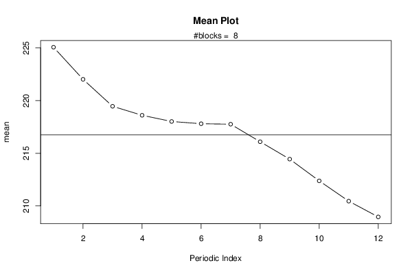
| R Software Module | rwasp_meanplot.wasp | ||||||||||||||||||||
| Title produced by software | Mean Plot | ||||||||||||||||||||
| Date of computation | Wed, 04 Mar 2015 18:15:18 +0000 | ||||||||||||||||||||
| Cite this page as follows | Statistical Computations at FreeStatistics.org, Office for Research Development and Education, URL https://freestatistics.org/blog/index.php?v=date/2015/Mar/04/t1425493002ph9xpq7dw634pm9.htm/, Retrieved Fri, 17 May 2024 02:40:16 +0000 | ||||||||||||||||||||
| Statistical Computations at FreeStatistics.org, Office for Research Development and Education, URL https://freestatistics.org/blog/index.php?pk=277891, Retrieved Fri, 17 May 2024 02:40:16 +0000 | |||||||||||||||||||||
| QR Codes: | |||||||||||||||||||||
|
| |||||||||||||||||||||
| Original text written by user: | |||||||||||||||||||||
| IsPrivate? | No (this computation is public) | ||||||||||||||||||||
| User-defined keywords | |||||||||||||||||||||
| Estimated Impact | 175 | ||||||||||||||||||||
Tree of Dependent Computations | |||||||||||||||||||||
| Family? (F = Feedback message, R = changed R code, M = changed R Module, P = changed Parameters, D = changed Data) | |||||||||||||||||||||
| - [Mean Plot] [] [2015-03-04 18:15:18] [006461bb825a57cb671d1f8ff85b37cb] [Current] | |||||||||||||||||||||
| Feedback Forum | |||||||||||||||||||||
Post a new message | |||||||||||||||||||||
Dataset | |||||||||||||||||||||
| Dataseries X: | |||||||||||||||||||||
299,81 299,01 296,82 296,67 296,95 296,80 296,80 295,93 293,77 291,02 288,61 284,55 284,55 278,14 273,28 270,14 268,36 267,15 267,15 265,47 261,75 256,51 252,98 251,17 251,17 244,27 240,54 238,92 237,47 235,91 235,91 231,41 224,94 222,19 219,06 217,83 217,83 216,89 213,84 212,90 213,98 215,31 215,31 214,09 213,71 211,54 209,40 207,33 207,33 202,75 200,26 198,99 198,82 198,43 198,43 195,68 195,45 193,65 191,38 189,71 189,71 185,49 183,01 182,38 181,60 182,13 182,13 180,81 180,25 179,84 178,50 178,11 178,11 178,10 177,52 177,34 175,53 176,01 175,94 175,47 175,48 173,76 173,74 173,65 172,00 171,50 170,41 171,50 171,43 170,69 170,40 169,90 170,21 170,55 169,98 169,34 | |||||||||||||||||||||
Tables (Output of Computation) | |||||||||||||||||||||
| |||||||||||||||||||||
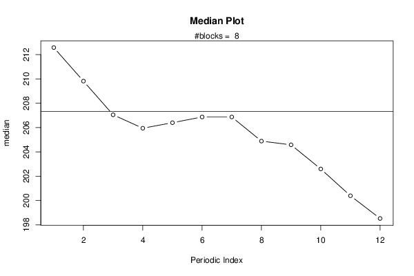
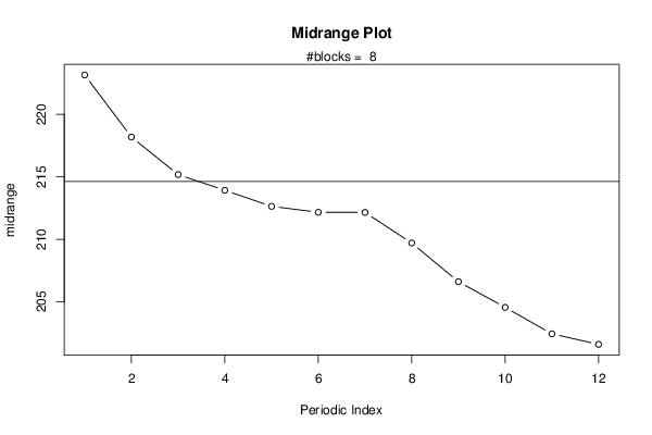
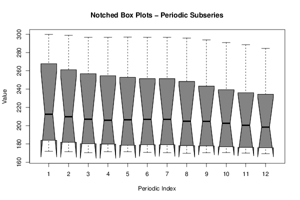
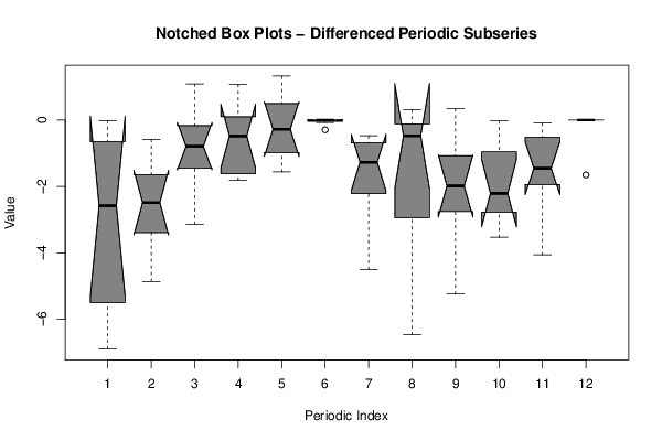
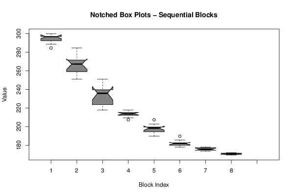
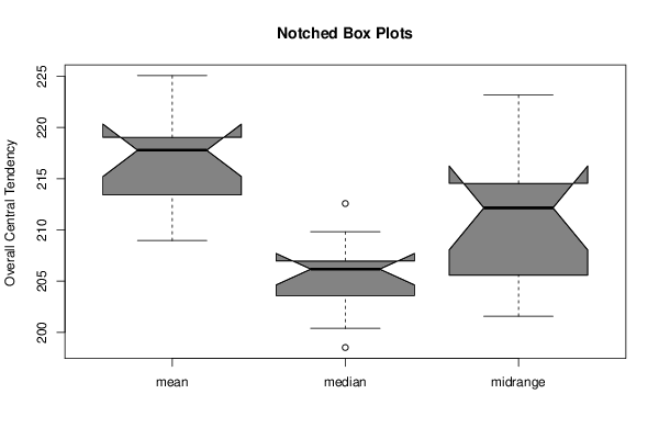
Figures (Output of Computation) | |||||||||||||||||||||
Input Parameters & R Code | |||||||||||||||||||||
| Parameters (Session): | |||||||||||||||||||||
| par1 = 12 ; | |||||||||||||||||||||
| Parameters (R input): | |||||||||||||||||||||
| par1 = 12 ; | |||||||||||||||||||||
| R code (references can be found in the software module): | |||||||||||||||||||||
par1 <- '12' | |||||||||||||||||||||