Repository of Reproducible Computations

Free Statistics

of Irreproducible Research!

Author's title

Author

*The author of this computation has been verified*

R Software Module

rwasp_autocorrelation.wasp

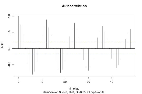
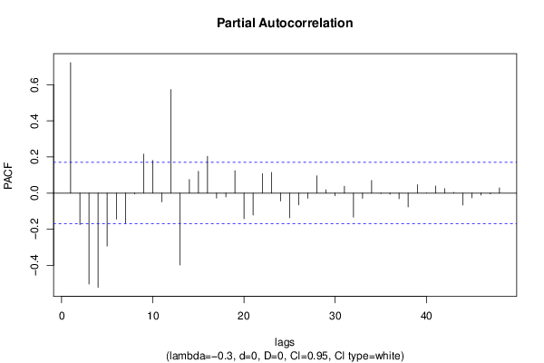
Title produced by software

(Partial) Autocorrelation Function

Date of computation

Mon, 19 Jan 2015 11:19:24 +0000

Cite this page as follows

Statistical Computations at FreeStatistics.org, Office for Research Development and Education, URL https://freestatistics.org/blog/index.php?v=date/2015/Jan/19/t142166639330rphywyofgk6p2.htm/, Retrieved Wed, 15 May 2024 17:29:30 +0000

Statistical Computations at FreeStatistics.org, Office for Research Development and Education, URL https://freestatistics.org/blog/index.php?pk=274455, Retrieved Wed, 15 May 2024 17:29:30 +0000

QR Codes:

Paste this QR Code to cite your computation.

Original text written by user:

IsPrivate?

No (this computation is public)

User-defined keywords

Estimated Impact

Family? (F = Feedback message, R = changed R code, M = changed R Module, P = changed Parameters, D = changed Data)

-     [One-Way-Between-Groups ANOVA- Free Statistics Software (Calculator)] [] [2010-11-01 13:37:53] [b98453cac15ba1066b407e146608df68]
- RMP   [One-Way-Between-Groups ANOVA- Free Statistics Software (Calculator)] [] [2014-10-21 08:05:52] [32b17a345b130fdf5cc88718ed94a974]
- RMPD      [(Partial) Autocorrelation Function] [vraag6(2)] [2015-01-19 11:19:24] [21b927ddce509724d48ffb8407994bd0] [Current]
- R P         [(Partial) Autocorrelation Function] [vraag6(3)] [2015-01-19 11:28:05] [7c87d1c7801dd67c2a0c90c2b6a05b3c] 
- RMP         [ARIMA Backward Selection] [vraag6(4)] [2015-01-19 11:30:25] [7c87d1c7801dd67c2a0c90c2b6a05b3c] 
- RMP         [ARIMA Forecasting] [vraag7] [2015-01-19 12:36:57] [7c87d1c7801dd67c2a0c90c2b6a05b3c] 

Feedback Forum

Post a new message

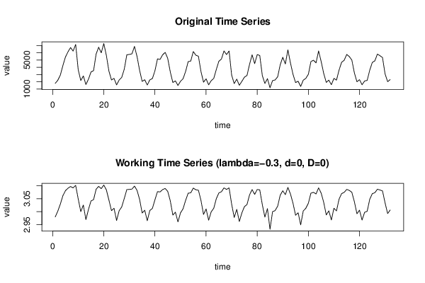
Dataseries X:

Download CSV

Histogram

Boxplots

Summary of computational transaction
Raw Input	view raw input (R code)
Raw Output	view raw output of R engine
Computing time	2 seconds
R Server	'Herman Ole Andreas Wold' @ wold.wessa.net

\begin{tabular}{lllllllll}
\hline
Summary of computational transaction \tabularnewline
Raw Input & view raw input (R code)  \tabularnewline
Raw Output & view raw output of R engine  \tabularnewline
Computing time & 2 seconds \tabularnewline
R Server & 'Herman Ole Andreas Wold' @ wold.wessa.net \tabularnewline
\hline
\end{tabular}
%Source: https://freestatistics.org/blog/index.php?pk=274455&T=0

[TABLE]
[ROW][C]Summary of computational transaction[/C][/ROW]
[ROW][C]Raw Input[/C][C]view raw input (R code) [/C][/ROW]
[ROW][C]Raw Output[/C][C]view raw output of R engine [/C][/ROW]
[ROW][C]Computing time[/C][C]2 seconds[/C][/ROW]
[ROW][C]R Server[/C][C]'Herman Ole Andreas Wold' @ wold.wessa.net[/C][/ROW]
[/TABLE]
Source: https://freestatistics.org/blog/index.php?pk=274455&T=0

Globally Unique Identifier (entire table): ba.freestatistics.org/blog/index.php?pk=274455&T=0

As an alternative you can also use a QR Code:

The GUIDs for individual cells are displayed in the table below:

Summary of computational transaction
Raw Input	view raw input (R code)
Raw Output	view raw output of R engine
Computing time	2 seconds
R Server	'Herman Ole Andreas Wold' @ wold.wessa.net

Autocorrelation Function
Time lag k	ACF(k)	T-STAT	P-value
1	0.722967	8.3063	0
2	0.439327	5.0475	1e-06
3	0.013706	0.1575	0.437558
4	-0.422897	-4.8587	2e-06
5	-0.703288	-8.0802	0
6	-0.802743	-9.2228	0
7	-0.710322	-8.161	0
8	-0.402032	-4.619	5e-06
9	0.022839	0.2624	0.396713
10	0.418749	4.8111	2e-06
11	0.6796	7.808	0
12	0.893024	10.2601	0
13	0.648969	7.4561	0
14	0.402628	4.6258	4e-06
15	0.001741	0.02	0.492038
16	-0.391166	-4.4942	8e-06
17	-0.641363	-7.3687	0
18	-0.744739	-8.5564	0
19	-0.651201	-7.4817	0
20	-0.370656	-4.2585	1.9e-05
21	0.00255	0.0293	0.488336
22	0.370001	4.251	2e-05
23	0.615069	7.0666	0
24	0.79488	9.1325	0
25	0.586192	6.7348	0
26	0.359364	4.1288	3.2e-05
27	-0.015459	-0.1776	0.429649
28	-0.35234	-4.0481	4.4e-05
29	-0.578119	-6.6421	0
30	-0.681917	-7.8346	0
31	-0.58376	-6.7069	0
32	-0.341002	-3.9178	7.1e-05
33	-0.003831	-0.044	0.48248
34	0.337077	3.8727	8.4e-05
35	0.545331	6.2654	0
36	0.698653	8.0269	0
37	0.52111	5.9871	0
38	0.308327	3.5424	0.000274
39	-0.018722	-0.2151	0.415011
40	-0.310742	-3.5702	0.000249
41	-0.515462	-5.9222	0
42	-0.605785	-6.9599	0
43	-0.510436	-5.8645	0
44	-0.306286	-3.519	0.000297
45	-0.002035	-0.0234	0.49069
46	0.295284	3.3926	0.000457
47	0.467999	5.3769	0
48	0.607043	6.9744	0

\begin{tabular}{lllllllll}
\hline
Autocorrelation Function \tabularnewline
Time lag k & ACF(k) & T-STAT & P-value \tabularnewline
1 & 0.722967 & 8.3063 & 0 \tabularnewline
2 & 0.439327 & 5.0475 & 1e-06 \tabularnewline
3 & 0.013706 & 0.1575 & 0.437558 \tabularnewline
4 & -0.422897 & -4.8587 & 2e-06 \tabularnewline
5 & -0.703288 & -8.0802 & 0 \tabularnewline
6 & -0.802743 & -9.2228 & 0 \tabularnewline
7 & -0.710322 & -8.161 & 0 \tabularnewline
8 & -0.402032 & -4.619 & 5e-06 \tabularnewline
9 & 0.022839 & 0.2624 & 0.396713 \tabularnewline
10 & 0.418749 & 4.8111 & 2e-06 \tabularnewline
11 & 0.6796 & 7.808 & 0 \tabularnewline
12 & 0.893024 & 10.2601 & 0 \tabularnewline
13 & 0.648969 & 7.4561 & 0 \tabularnewline
14 & 0.402628 & 4.6258 & 4e-06 \tabularnewline
15 & 0.001741 & 0.02 & 0.492038 \tabularnewline
16 & -0.391166 & -4.4942 & 8e-06 \tabularnewline
17 & -0.641363 & -7.3687 & 0 \tabularnewline
18 & -0.744739 & -8.5564 & 0 \tabularnewline
19 & -0.651201 & -7.4817 & 0 \tabularnewline
20 & -0.370656 & -4.2585 & 1.9e-05 \tabularnewline
21 & 0.00255 & 0.0293 & 0.488336 \tabularnewline
22 & 0.370001 & 4.251 & 2e-05 \tabularnewline
23 & 0.615069 & 7.0666 & 0 \tabularnewline
24 & 0.79488 & 9.1325 & 0 \tabularnewline
25 & 0.586192 & 6.7348 & 0 \tabularnewline
26 & 0.359364 & 4.1288 & 3.2e-05 \tabularnewline
27 & -0.015459 & -0.1776 & 0.429649 \tabularnewline
28 & -0.35234 & -4.0481 & 4.4e-05 \tabularnewline
29 & -0.578119 & -6.6421 & 0 \tabularnewline
30 & -0.681917 & -7.8346 & 0 \tabularnewline
31 & -0.58376 & -6.7069 & 0 \tabularnewline
32 & -0.341002 & -3.9178 & 7.1e-05 \tabularnewline
33 & -0.003831 & -0.044 & 0.48248 \tabularnewline
34 & 0.337077 & 3.8727 & 8.4e-05 \tabularnewline
35 & 0.545331 & 6.2654 & 0 \tabularnewline
36 & 0.698653 & 8.0269 & 0 \tabularnewline
37 & 0.52111 & 5.9871 & 0 \tabularnewline
38 & 0.308327 & 3.5424 & 0.000274 \tabularnewline
39 & -0.018722 & -0.2151 & 0.415011 \tabularnewline
40 & -0.310742 & -3.5702 & 0.000249 \tabularnewline
41 & -0.515462 & -5.9222 & 0 \tabularnewline
42 & -0.605785 & -6.9599 & 0 \tabularnewline
43 & -0.510436 & -5.8645 & 0 \tabularnewline
44 & -0.306286 & -3.519 & 0.000297 \tabularnewline
45 & -0.002035 & -0.0234 & 0.49069 \tabularnewline
46 & 0.295284 & 3.3926 & 0.000457 \tabularnewline
47 & 0.467999 & 5.3769 & 0 \tabularnewline
48 & 0.607043 & 6.9744 & 0 \tabularnewline
\hline
\end{tabular}
%Source: https://freestatistics.org/blog/index.php?pk=274455&T=1

[TABLE]
[ROW][C]Autocorrelation Function[/C][/ROW]
[ROW][C]Time lag k[/C][C]ACF(k)[/C][C]T-STAT[/C][C]P-value[/C][/ROW]
[ROW][C]1[/C][C]0.722967[/C][C]8.3063[/C][C]0[/C][/ROW]
[ROW][C]2[/C][C]0.439327[/C][C]5.0475[/C][C]1e-06[/C][/ROW]
[ROW][C]3[/C][C]0.013706[/C][C]0.1575[/C][C]0.437558[/C][/ROW]
[ROW][C]4[/C][C]-0.422897[/C][C]-4.8587[/C][C]2e-06[/C][/ROW]
[ROW][C]5[/C][C]-0.703288[/C][C]-8.0802[/C][C]0[/C][/ROW]
[ROW][C]6[/C][C]-0.802743[/C][C]-9.2228[/C][C]0[/C][/ROW]
[ROW][C]7[/C][C]-0.710322[/C][C]-8.161[/C][C]0[/C][/ROW]
[ROW][C]8[/C][C]-0.402032[/C][C]-4.619[/C][C]5e-06[/C][/ROW]
[ROW][C]9[/C][C]0.022839[/C][C]0.2624[/C][C]0.396713[/C][/ROW]
[ROW][C]10[/C][C]0.418749[/C][C]4.8111[/C][C]2e-06[/C][/ROW]
[ROW][C]11[/C][C]0.6796[/C][C]7.808[/C][C]0[/C][/ROW]
[ROW][C]12[/C][C]0.893024[/C][C]10.2601[/C][C]0[/C][/ROW]
[ROW][C]13[/C][C]0.648969[/C][C]7.4561[/C][C]0[/C][/ROW]
[ROW][C]14[/C][C]0.402628[/C][C]4.6258[/C][C]4e-06[/C][/ROW]
[ROW][C]15[/C][C]0.001741[/C][C]0.02[/C][C]0.492038[/C][/ROW]
[ROW][C]16[/C][C]-0.391166[/C][C]-4.4942[/C][C]8e-06[/C][/ROW]
[ROW][C]17[/C][C]-0.641363[/C][C]-7.3687[/C][C]0[/C][/ROW]
[ROW][C]18[/C][C]-0.744739[/C][C]-8.5564[/C][C]0[/C][/ROW]
[ROW][C]19[/C][C]-0.651201[/C][C]-7.4817[/C][C]0[/C][/ROW]
[ROW][C]20[/C][C]-0.370656[/C][C]-4.2585[/C][C]1.9e-05[/C][/ROW]
[ROW][C]21[/C][C]0.00255[/C][C]0.0293[/C][C]0.488336[/C][/ROW]
[ROW][C]22[/C][C]0.370001[/C][C]4.251[/C][C]2e-05[/C][/ROW]
[ROW][C]23[/C][C]0.615069[/C][C]7.0666[/C][C]0[/C][/ROW]
[ROW][C]24[/C][C]0.79488[/C][C]9.1325[/C][C]0[/C][/ROW]
[ROW][C]25[/C][C]0.586192[/C][C]6.7348[/C][C]0[/C][/ROW]
[ROW][C]26[/C][C]0.359364[/C][C]4.1288[/C][C]3.2e-05[/C][/ROW]
[ROW][C]27[/C][C]-0.015459[/C][C]-0.1776[/C][C]0.429649[/C][/ROW]
[ROW][C]28[/C][C]-0.35234[/C][C]-4.0481[/C][C]4.4e-05[/C][/ROW]
[ROW][C]29[/C][C]-0.578119[/C][C]-6.6421[/C][C]0[/C][/ROW]
[ROW][C]30[/C][C]-0.681917[/C][C]-7.8346[/C][C]0[/C][/ROW]
[ROW][C]31[/C][C]-0.58376[/C][C]-6.7069[/C][C]0[/C][/ROW]
[ROW][C]32[/C][C]-0.341002[/C][C]-3.9178[/C][C]7.1e-05[/C][/ROW]
[ROW][C]33[/C][C]-0.003831[/C][C]-0.044[/C][C]0.48248[/C][/ROW]
[ROW][C]34[/C][C]0.337077[/C][C]3.8727[/C][C]8.4e-05[/C][/ROW]
[ROW][C]35[/C][C]0.545331[/C][C]6.2654[/C][C]0[/C][/ROW]
[ROW][C]36[/C][C]0.698653[/C][C]8.0269[/C][C]0[/C][/ROW]
[ROW][C]37[/C][C]0.52111[/C][C]5.9871[/C][C]0[/C][/ROW]
[ROW][C]38[/C][C]0.308327[/C][C]3.5424[/C][C]0.000274[/C][/ROW]
[ROW][C]39[/C][C]-0.018722[/C][C]-0.2151[/C][C]0.415011[/C][/ROW]
[ROW][C]40[/C][C]-0.310742[/C][C]-3.5702[/C][C]0.000249[/C][/ROW]
[ROW][C]41[/C][C]-0.515462[/C][C]-5.9222[/C][C]0[/C][/ROW]
[ROW][C]42[/C][C]-0.605785[/C][C]-6.9599[/C][C]0[/C][/ROW]
[ROW][C]43[/C][C]-0.510436[/C][C]-5.8645[/C][C]0[/C][/ROW]
[ROW][C]44[/C][C]-0.306286[/C][C]-3.519[/C][C]0.000297[/C][/ROW]
[ROW][C]45[/C][C]-0.002035[/C][C]-0.0234[/C][C]0.49069[/C][/ROW]
[ROW][C]46[/C][C]0.295284[/C][C]3.3926[/C][C]0.000457[/C][/ROW]
[ROW][C]47[/C][C]0.467999[/C][C]5.3769[/C][C]0[/C][/ROW]
[ROW][C]48[/C][C]0.607043[/C][C]6.9744[/C][C]0[/C][/ROW]
[/TABLE]
Source: https://freestatistics.org/blog/index.php?pk=274455&T=1

Globally Unique Identifier (entire table): ba.freestatistics.org/blog/index.php?pk=274455&T=1

As an alternative you can also use a QR Code:

The GUIDs for individual cells are displayed in the table below:

Autocorrelation Function
Time lag k	ACF(k)	T-STAT	P-value
1	0.722967	8.3063	0
2	0.439327	5.0475	1e-06
3	0.013706	0.1575	0.437558
4	-0.422897	-4.8587	2e-06
5	-0.703288	-8.0802	0
6	-0.802743	-9.2228	0
7	-0.710322	-8.161	0
8	-0.402032	-4.619	5e-06
9	0.022839	0.2624	0.396713
10	0.418749	4.8111	2e-06
11	0.6796	7.808	0
12	0.893024	10.2601	0
13	0.648969	7.4561	0
14	0.402628	4.6258	4e-06
15	0.001741	0.02	0.492038
16	-0.391166	-4.4942	8e-06
17	-0.641363	-7.3687	0
18	-0.744739	-8.5564	0
19	-0.651201	-7.4817	0
20	-0.370656	-4.2585	1.9e-05
21	0.00255	0.0293	0.488336
22	0.370001	4.251	2e-05
23	0.615069	7.0666	0
24	0.79488	9.1325	0
25	0.586192	6.7348	0
26	0.359364	4.1288	3.2e-05
27	-0.015459	-0.1776	0.429649
28	-0.35234	-4.0481	4.4e-05
29	-0.578119	-6.6421	0
30	-0.681917	-7.8346	0
31	-0.58376	-6.7069	0
32	-0.341002	-3.9178	7.1e-05
33	-0.003831	-0.044	0.48248
34	0.337077	3.8727	8.4e-05
35	0.545331	6.2654	0
36	0.698653	8.0269	0
37	0.52111	5.9871	0
38	0.308327	3.5424	0.000274
39	-0.018722	-0.2151	0.415011
40	-0.310742	-3.5702	0.000249
41	-0.515462	-5.9222	0
42	-0.605785	-6.9599	0
43	-0.510436	-5.8645	0
44	-0.306286	-3.519	0.000297
45	-0.002035	-0.0234	0.49069
46	0.295284	3.3926	0.000457
47	0.467999	5.3769	0
48	0.607043	6.9744	0

Partial Autocorrelation Function
Time lag k	PACF(k)	T-STAT	P-value
1	0.722967	8.3063	0
2	-0.17463	-2.0063	0.023431
3	-0.503771	-5.7879	0
4	-0.522268	-6.0004	0
5	-0.293355	-3.3704	0.000492
6	-0.144237	-1.6572	0.049931
7	-0.166105	-1.9084	0.029256
8	-0.004914	-0.0565	0.477531
9	0.215653	2.4777	0.007244
10	0.180431	2.073	0.020059
11	-0.04868	-0.5593	0.288455
12	0.573772	6.5921	0
13	-0.398458	-4.5779	5e-06
14	0.075408	0.8664	0.193931
15	0.120354	1.3828	0.084537
16	0.203801	2.3415	0.010352
17	-0.027296	-0.3136	0.377158
18	-0.021598	-0.2481	0.402206
19	0.12419	1.4268	0.077995
20	-0.141936	-1.6307	0.052666
21	-0.121695	-1.3982	0.082203
22	0.107533	1.2355	0.109427
23	0.1148	1.319	0.094734
24	-0.043588	-0.5008	0.308675
25	-0.136728	-1.5709	0.059302
26	-0.064971	-0.7465	0.228358
27	-0.028918	-0.3322	0.370115
28	0.095247	1.0943	0.137906
29	0.018482	0.2123	0.416084
30	-0.015367	-0.1765	0.430067
31	0.038251	0.4395	0.330521
32	-0.133398	-1.5326	0.06388
33	-0.02862	-0.3288	0.371408
34	0.069727	0.8011	0.212255
35	-0.002661	-0.0306	0.48783
36	-0.005986	-0.0688	0.472638
37	-0.031171	-0.3581	0.360409
38	-0.076814	-0.8825	0.189548
39	0.046927	0.5392	0.295345
40	0.000119	0.0014	0.499458
41	0.039302	0.4515	0.326169
42	0.024674	0.2835	0.388625
43	0.004144	0.0476	0.481047
44	-0.065986	-0.7581	0.224865
45	-0.026405	-0.3034	0.381043
46	-0.011106	-0.1276	0.449332
47	-0.004339	-0.0499	0.480157
48	0.028788	0.3307	0.370679

\begin{tabular}{lllllllll}
\hline
Partial Autocorrelation Function \tabularnewline
Time lag k & PACF(k) & T-STAT & P-value \tabularnewline
1 & 0.722967 & 8.3063 & 0 \tabularnewline
2 & -0.17463 & -2.0063 & 0.023431 \tabularnewline
3 & -0.503771 & -5.7879 & 0 \tabularnewline
4 & -0.522268 & -6.0004 & 0 \tabularnewline
5 & -0.293355 & -3.3704 & 0.000492 \tabularnewline
6 & -0.144237 & -1.6572 & 0.049931 \tabularnewline
7 & -0.166105 & -1.9084 & 0.029256 \tabularnewline
8 & -0.004914 & -0.0565 & 0.477531 \tabularnewline
9 & 0.215653 & 2.4777 & 0.007244 \tabularnewline
10 & 0.180431 & 2.073 & 0.020059 \tabularnewline
11 & -0.04868 & -0.5593 & 0.288455 \tabularnewline
12 & 0.573772 & 6.5921 & 0 \tabularnewline
13 & -0.398458 & -4.5779 & 5e-06 \tabularnewline
14 & 0.075408 & 0.8664 & 0.193931 \tabularnewline
15 & 0.120354 & 1.3828 & 0.084537 \tabularnewline
16 & 0.203801 & 2.3415 & 0.010352 \tabularnewline
17 & -0.027296 & -0.3136 & 0.377158 \tabularnewline
18 & -0.021598 & -0.2481 & 0.402206 \tabularnewline
19 & 0.12419 & 1.4268 & 0.077995 \tabularnewline
20 & -0.141936 & -1.6307 & 0.052666 \tabularnewline
21 & -0.121695 & -1.3982 & 0.082203 \tabularnewline
22 & 0.107533 & 1.2355 & 0.109427 \tabularnewline
23 & 0.1148 & 1.319 & 0.094734 \tabularnewline
24 & -0.043588 & -0.5008 & 0.308675 \tabularnewline
25 & -0.136728 & -1.5709 & 0.059302 \tabularnewline
26 & -0.064971 & -0.7465 & 0.228358 \tabularnewline
27 & -0.028918 & -0.3322 & 0.370115 \tabularnewline
28 & 0.095247 & 1.0943 & 0.137906 \tabularnewline
29 & 0.018482 & 0.2123 & 0.416084 \tabularnewline
30 & -0.015367 & -0.1765 & 0.430067 \tabularnewline
31 & 0.038251 & 0.4395 & 0.330521 \tabularnewline
32 & -0.133398 & -1.5326 & 0.06388 \tabularnewline
33 & -0.02862 & -0.3288 & 0.371408 \tabularnewline
34 & 0.069727 & 0.8011 & 0.212255 \tabularnewline
35 & -0.002661 & -0.0306 & 0.48783 \tabularnewline
36 & -0.005986 & -0.0688 & 0.472638 \tabularnewline
37 & -0.031171 & -0.3581 & 0.360409 \tabularnewline
38 & -0.076814 & -0.8825 & 0.189548 \tabularnewline
39 & 0.046927 & 0.5392 & 0.295345 \tabularnewline
40 & 0.000119 & 0.0014 & 0.499458 \tabularnewline
41 & 0.039302 & 0.4515 & 0.326169 \tabularnewline
42 & 0.024674 & 0.2835 & 0.388625 \tabularnewline
43 & 0.004144 & 0.0476 & 0.481047 \tabularnewline
44 & -0.065986 & -0.7581 & 0.224865 \tabularnewline
45 & -0.026405 & -0.3034 & 0.381043 \tabularnewline
46 & -0.011106 & -0.1276 & 0.449332 \tabularnewline
47 & -0.004339 & -0.0499 & 0.480157 \tabularnewline
48 & 0.028788 & 0.3307 & 0.370679 \tabularnewline
\hline
\end{tabular}
%Source: https://freestatistics.org/blog/index.php?pk=274455&T=2

[TABLE]
[ROW][C]Partial Autocorrelation Function[/C][/ROW]
[ROW][C]Time lag k[/C][C]PACF(k)[/C][C]T-STAT[/C][C]P-value[/C][/ROW]
[ROW][C]1[/C][C]0.722967[/C][C]8.3063[/C][C]0[/C][/ROW]
[ROW][C]2[/C][C]-0.17463[/C][C]-2.0063[/C][C]0.023431[/C][/ROW]
[ROW][C]3[/C][C]-0.503771[/C][C]-5.7879[/C][C]0[/C][/ROW]
[ROW][C]4[/C][C]-0.522268[/C][C]-6.0004[/C][C]0[/C][/ROW]
[ROW][C]5[/C][C]-0.293355[/C][C]-3.3704[/C][C]0.000492[/C][/ROW]
[ROW][C]6[/C][C]-0.144237[/C][C]-1.6572[/C][C]0.049931[/C][/ROW]
[ROW][C]7[/C][C]-0.166105[/C][C]-1.9084[/C][C]0.029256[/C][/ROW]
[ROW][C]8[/C][C]-0.004914[/C][C]-0.0565[/C][C]0.477531[/C][/ROW]
[ROW][C]9[/C][C]0.215653[/C][C]2.4777[/C][C]0.007244[/C][/ROW]
[ROW][C]10[/C][C]0.180431[/C][C]2.073[/C][C]0.020059[/C][/ROW]
[ROW][C]11[/C][C]-0.04868[/C][C]-0.5593[/C][C]0.288455[/C][/ROW]
[ROW][C]12[/C][C]0.573772[/C][C]6.5921[/C][C]0[/C][/ROW]
[ROW][C]13[/C][C]-0.398458[/C][C]-4.5779[/C][C]5e-06[/C][/ROW]
[ROW][C]14[/C][C]0.075408[/C][C]0.8664[/C][C]0.193931[/C][/ROW]
[ROW][C]15[/C][C]0.120354[/C][C]1.3828[/C][C]0.084537[/C][/ROW]
[ROW][C]16[/C][C]0.203801[/C][C]2.3415[/C][C]0.010352[/C][/ROW]
[ROW][C]17[/C][C]-0.027296[/C][C]-0.3136[/C][C]0.377158[/C][/ROW]
[ROW][C]18[/C][C]-0.021598[/C][C]-0.2481[/C][C]0.402206[/C][/ROW]
[ROW][C]19[/C][C]0.12419[/C][C]1.4268[/C][C]0.077995[/C][/ROW]
[ROW][C]20[/C][C]-0.141936[/C][C]-1.6307[/C][C]0.052666[/C][/ROW]
[ROW][C]21[/C][C]-0.121695[/C][C]-1.3982[/C][C]0.082203[/C][/ROW]
[ROW][C]22[/C][C]0.107533[/C][C]1.2355[/C][C]0.109427[/C][/ROW]
[ROW][C]23[/C][C]0.1148[/C][C]1.319[/C][C]0.094734[/C][/ROW]
[ROW][C]24[/C][C]-0.043588[/C][C]-0.5008[/C][C]0.308675[/C][/ROW]
[ROW][C]25[/C][C]-0.136728[/C][C]-1.5709[/C][C]0.059302[/C][/ROW]
[ROW][C]26[/C][C]-0.064971[/C][C]-0.7465[/C][C]0.228358[/C][/ROW]
[ROW][C]27[/C][C]-0.028918[/C][C]-0.3322[/C][C]0.370115[/C][/ROW]
[ROW][C]28[/C][C]0.095247[/C][C]1.0943[/C][C]0.137906[/C][/ROW]
[ROW][C]29[/C][C]0.018482[/C][C]0.2123[/C][C]0.416084[/C][/ROW]
[ROW][C]30[/C][C]-0.015367[/C][C]-0.1765[/C][C]0.430067[/C][/ROW]
[ROW][C]31[/C][C]0.038251[/C][C]0.4395[/C][C]0.330521[/C][/ROW]
[ROW][C]32[/C][C]-0.133398[/C][C]-1.5326[/C][C]0.06388[/C][/ROW]
[ROW][C]33[/C][C]-0.02862[/C][C]-0.3288[/C][C]0.371408[/C][/ROW]
[ROW][C]34[/C][C]0.069727[/C][C]0.8011[/C][C]0.212255[/C][/ROW]
[ROW][C]35[/C][C]-0.002661[/C][C]-0.0306[/C][C]0.48783[/C][/ROW]
[ROW][C]36[/C][C]-0.005986[/C][C]-0.0688[/C][C]0.472638[/C][/ROW]
[ROW][C]37[/C][C]-0.031171[/C][C]-0.3581[/C][C]0.360409[/C][/ROW]
[ROW][C]38[/C][C]-0.076814[/C][C]-0.8825[/C][C]0.189548[/C][/ROW]
[ROW][C]39[/C][C]0.046927[/C][C]0.5392[/C][C]0.295345[/C][/ROW]
[ROW][C]40[/C][C]0.000119[/C][C]0.0014[/C][C]0.499458[/C][/ROW]
[ROW][C]41[/C][C]0.039302[/C][C]0.4515[/C][C]0.326169[/C][/ROW]
[ROW][C]42[/C][C]0.024674[/C][C]0.2835[/C][C]0.388625[/C][/ROW]
[ROW][C]43[/C][C]0.004144[/C][C]0.0476[/C][C]0.481047[/C][/ROW]
[ROW][C]44[/C][C]-0.065986[/C][C]-0.7581[/C][C]0.224865[/C][/ROW]
[ROW][C]45[/C][C]-0.026405[/C][C]-0.3034[/C][C]0.381043[/C][/ROW]
[ROW][C]46[/C][C]-0.011106[/C][C]-0.1276[/C][C]0.449332[/C][/ROW]
[ROW][C]47[/C][C]-0.004339[/C][C]-0.0499[/C][C]0.480157[/C][/ROW]
[ROW][C]48[/C][C]0.028788[/C][C]0.3307[/C][C]0.370679[/C][/ROW]
[/TABLE]
Source: https://freestatistics.org/blog/index.php?pk=274455&T=2

Globally Unique Identifier (entire table): ba.freestatistics.org/blog/index.php?pk=274455&T=2

As an alternative you can also use a QR Code:

The GUIDs for individual cells are displayed in the table below:

Partial Autocorrelation Function
Time lag k	PACF(k)	T-STAT	P-value
1	0.722967	8.3063	0
2	-0.17463	-2.0063	0.023431
3	-0.503771	-5.7879	0
4	-0.522268	-6.0004	0
5	-0.293355	-3.3704	0.000492
6	-0.144237	-1.6572	0.049931
7	-0.166105	-1.9084	0.029256
8	-0.004914	-0.0565	0.477531
9	0.215653	2.4777	0.007244
10	0.180431	2.073	0.020059
11	-0.04868	-0.5593	0.288455
12	0.573772	6.5921	0
13	-0.398458	-4.5779	5e-06
14	0.075408	0.8664	0.193931
15	0.120354	1.3828	0.084537
16	0.203801	2.3415	0.010352
17	-0.027296	-0.3136	0.377158
18	-0.021598	-0.2481	0.402206
19	0.12419	1.4268	0.077995
20	-0.141936	-1.6307	0.052666
21	-0.121695	-1.3982	0.082203
22	0.107533	1.2355	0.109427
23	0.1148	1.319	0.094734
24	-0.043588	-0.5008	0.308675
25	-0.136728	-1.5709	0.059302
26	-0.064971	-0.7465	0.228358
27	-0.028918	-0.3322	0.370115
28	0.095247	1.0943	0.137906
29	0.018482	0.2123	0.416084
30	-0.015367	-0.1765	0.430067
31	0.038251	0.4395	0.330521
32	-0.133398	-1.5326	0.06388
33	-0.02862	-0.3288	0.371408
34	0.069727	0.8011	0.212255
35	-0.002661	-0.0306	0.48783
36	-0.005986	-0.0688	0.472638
37	-0.031171	-0.3581	0.360409
38	-0.076814	-0.8825	0.189548
39	0.046927	0.5392	0.295345
40	0.000119	0.0014	0.499458
41	0.039302	0.4515	0.326169
42	0.024674	0.2835	0.388625
43	0.004144	0.0476	0.481047
44	-0.065986	-0.7581	0.224865
45	-0.026405	-0.3034	0.381043
46	-0.011106	-0.1276	0.449332
47	-0.004339	-0.0499	0.480157
48	0.028788	0.3307	0.370679

Figure 1

PNG link

Postscript link

PDF link

Figure 2

PNG link

Postscript link

PDF link

Figure 3

PNG link

Postscript link

PDF link

Parameters (Session):

par1 = 48 ; par2 = -0.3 ; par3 = 0 ; par4 = 0 ; par5 = 12 ; par6 = White Noise ; par7 = 0.95 ;

Parameters (R input):

par1 = 48 ; par2 = -0.3 ; par3 = 0 ; par4 = 0 ; par5 = 12 ; par6 = White Noise ; par7 = 0.95 ; par8 = ;

R code (references can be found in the software module):

if (par1 == 'Default') {
par1 = 10*log10(length(x))
} else {
par1 <- as.numeric(par1)
}
par2 <- as.numeric(par2)
par3 <- as.numeric(par3)
par4 <- as.numeric(par4)
par5 <- as.numeric(par5)
if (par6 == 'White Noise') par6 <- 'white' else par6 <- 'ma'
par7 <- as.numeric(par7)
if (par8 != '') par8 <- as.numeric(par8)
ox <- x
if (par8 == '') {
if (par2 == 0) {
x <- log(x)
} else {
x <- (x ^ par2 - 1) / par2
}
} else {
x <- log(x,base=par8)
}
if (par3 > 0) x <- diff(x,lag=1,difference=par3)
if (par4 > 0) x <- diff(x,lag=par5,difference=par4)
bitmap(file='picts.png')
op <- par(mfrow=c(2,1))
plot(ox,type='l',main='Original Time Series',xlab='time',ylab='value')
if (par8=='') {
mytitle <- paste('Working Time Series (lambda=',par2,', d=',par3,', D=',par4,')',sep='')
mysub <- paste('(lambda=',par2,', d=',par3,', D=',par4,', CI=', par7, ', CI type=',par6,')',sep='')
} else {
mytitle <- paste('Working Time Series (base=',par8,', d=',par3,', D=',par4,')',sep='')
mysub <- paste('(base=',par8,', d=',par3,', D=',par4,', CI=', par7, ', CI type=',par6,')',sep='')
}
plot(x,type='l', main=mytitle,xlab='time',ylab='value')
par(op)
dev.off()
bitmap(file='pic1.png')
racf <- acf(x, par1, main='Autocorrelation', xlab='time lag', ylab='ACF', ci.type=par6, ci=par7, sub=mysub)
dev.off()
bitmap(file='pic2.png')
rpacf <- pacf(x,par1,main='Partial Autocorrelation',xlab='lags',ylab='PACF',sub=mysub)
dev.off()
(myacf <- c(racf$acf))
(mypacf <- c(rpacf$acf))
lengthx <- length(x)
sqrtn <- sqrt(lengthx)
load(file='createtable')
a<-table.start()
a<-table.row.start(a)
a<-table.element(a,'Autocorrelation Function',4,TRUE)
a<-table.row.end(a)
a<-table.row.start(a)
a<-table.element(a,'Time lag k',header=TRUE)
a<-table.element(a,hyperlink('basics.htm','ACF(k)','click here for more information about the Autocorrelation Function'),header=TRUE)
a<-table.element(a,'T-STAT',header=TRUE)
a<-table.element(a,'P-value',header=TRUE)
a<-table.row.end(a)
for (i in 2:(par1+1)) {
a<-table.row.start(a)
a<-table.element(a,i-1,header=TRUE)
a<-table.element(a,round(myacf[i],6))
mytstat <- myacf[i]*sqrtn
a<-table.element(a,round(mytstat,4))
a<-table.element(a,round(1-pt(abs(mytstat),lengthx),6))
a<-table.row.end(a)
}
a<-table.end(a)
table.save(a,file='mytable.tab')
a<-table.start()
a<-table.row.start(a)
a<-table.element(a,'Partial Autocorrelation Function',4,TRUE)
a<-table.row.end(a)
a<-table.row.start(a)
a<-table.element(a,'Time lag k',header=TRUE)
a<-table.element(a,hyperlink('basics.htm','PACF(k)','click here for more information about the Partial Autocorrelation Function'),header=TRUE)
a<-table.element(a,'T-STAT',header=TRUE)
a<-table.element(a,'P-value',header=TRUE)
a<-table.row.end(a)
for (i in 1:par1) {
a<-table.row.start(a)
a<-table.element(a,i,header=TRUE)
a<-table.element(a,round(mypacf[i],6))
mytstat <- mypacf[i]*sqrtn
a<-table.element(a,round(mytstat,4))
a<-table.element(a,round(1-pt(abs(mytstat),lengthx),6))
a<-table.row.end(a)
}
a<-table.end(a)
table.save(a,file='mytable1.tab')

Free Statistics

Description of Statistical Computation

Tree of Dependent Computations

Dataset

Tables (Output of Computation)

Figures (Output of Computation)

Input Parameters & R Code