Free Statistics
of Irreproducible Research!
Description of Statistical Computation | |||||||||||||||||||||||||||||||||||||||||||||||||||||||||||||||||||||||||||||||||
|---|---|---|---|---|---|---|---|---|---|---|---|---|---|---|---|---|---|---|---|---|---|---|---|---|---|---|---|---|---|---|---|---|---|---|---|---|---|---|---|---|---|---|---|---|---|---|---|---|---|---|---|---|---|---|---|---|---|---|---|---|---|---|---|---|---|---|---|---|---|---|---|---|---|---|---|---|---|---|---|---|---|
| Author's title | |||||||||||||||||||||||||||||||||||||||||||||||||||||||||||||||||||||||||||||||||
| Author | *Unverified author* | ||||||||||||||||||||||||||||||||||||||||||||||||||||||||||||||||||||||||||||||||
| R Software Module | rwasp_bootstrapplot.wasp | ||||||||||||||||||||||||||||||||||||||||||||||||||||||||||||||||||||||||||||||||
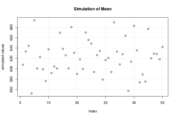
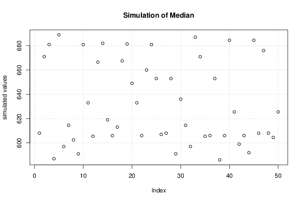
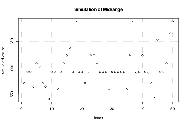
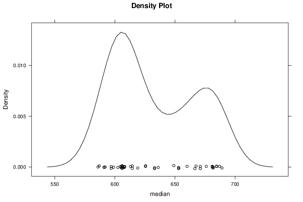
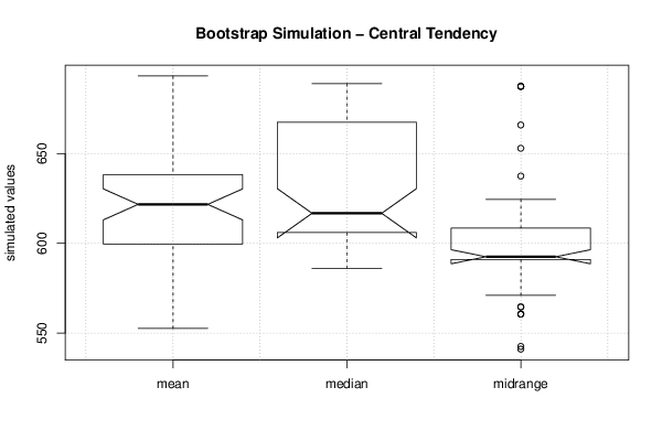
| Title produced by software | Blocked Bootstrap Plot - Central Tendency | ||||||||||||||||||||||||||||||||||||||||||||||||||||||||||||||||||||||||||||||||
| Date of computation | Tue, 06 Jan 2015 10:19:09 +0000 | ||||||||||||||||||||||||||||||||||||||||||||||||||||||||||||||||||||||||||||||||
| Cite this page as follows | Statistical Computations at FreeStatistics.org, Office for Research Development and Education, URL https://freestatistics.org/blog/index.php?v=date/2015/Jan/06/t14205396112znvrgxvs56jkpd.htm/, Retrieved Wed, 15 May 2024 10:30:47 +0000 | ||||||||||||||||||||||||||||||||||||||||||||||||||||||||||||||||||||||||||||||||
| Statistical Computations at FreeStatistics.org, Office for Research Development and Education, URL https://freestatistics.org/blog/index.php?pk=271994, Retrieved Wed, 15 May 2024 10:30:47 +0000 | |||||||||||||||||||||||||||||||||||||||||||||||||||||||||||||||||||||||||||||||||
| QR Codes: | |||||||||||||||||||||||||||||||||||||||||||||||||||||||||||||||||||||||||||||||||
|
| |||||||||||||||||||||||||||||||||||||||||||||||||||||||||||||||||||||||||||||||||
| Original text written by user: | |||||||||||||||||||||||||||||||||||||||||||||||||||||||||||||||||||||||||||||||||
| IsPrivate? | No (this computation is public) | ||||||||||||||||||||||||||||||||||||||||||||||||||||||||||||||||||||||||||||||||
| User-defined keywords | |||||||||||||||||||||||||||||||||||||||||||||||||||||||||||||||||||||||||||||||||
| Estimated Impact | 147 | ||||||||||||||||||||||||||||||||||||||||||||||||||||||||||||||||||||||||||||||||
Tree of Dependent Computations | |||||||||||||||||||||||||||||||||||||||||||||||||||||||||||||||||||||||||||||||||
| Family? (F = Feedback message, R = changed R code, M = changed R Module, P = changed Parameters, D = changed Data) | |||||||||||||||||||||||||||||||||||||||||||||||||||||||||||||||||||||||||||||||||
| - [Harrell-Davis Quantiles] [] [2015-01-05 16:01:40] [a8f6a7eeade7f89f597831d453788737] - D [Harrell-Davis Quantiles] [] [2015-01-05 16:10:43] [a8f6a7eeade7f89f597831d453788737] - RM [(Partial) Autocorrelation Function] [] [2015-01-06 09:12:41] [a8f6a7eeade7f89f597831d453788737] - RM D [Bootstrap Plot - Central Tendency] [] [2015-01-06 09:27:21] [a8f6a7eeade7f89f597831d453788737] - RM D [Blocked Bootstrap Plot - Central Tendency] [] [2015-01-06 10:19:09] [12470bd120139be5e23c611c04d9c0dc] [Current] - RM D [Variability] [] [2015-01-06 11:02:39] [a8f6a7eeade7f89f597831d453788737] - RM D [Standard Deviation Plot] [] [2015-01-06 11:07:17] [a8f6a7eeade7f89f597831d453788737] - RM D [Standard Deviation-Mean Plot] [] [2015-01-06 11:32:43] [a8f6a7eeade7f89f597831d453788737] - RM [Variability] [] [2015-01-06 11:43:50] [a8f6a7eeade7f89f597831d453788737] - RM [Standard Deviation Plot] [] [2015-01-06 11:48:58] [a8f6a7eeade7f89f597831d453788737] - RM [Standard Deviation-Mean Plot] [] [2015-01-06 12:01:28] [a8f6a7eeade7f89f597831d453788737] - RM D [Classical Decomposition] [] [2015-01-06 12:12:48] [a8f6a7eeade7f89f597831d453788737] - RM [Exponential Smoothing] [] [2015-01-06 12:25:54] [a8f6a7eeade7f89f597831d453788737] - RM D [Exponential Smoothing] [] [2015-01-06 12:34:40] [a8f6a7eeade7f89f597831d453788737] | |||||||||||||||||||||||||||||||||||||||||||||||||||||||||||||||||||||||||||||||||
| Feedback Forum | |||||||||||||||||||||||||||||||||||||||||||||||||||||||||||||||||||||||||||||||||
Post a new message | |||||||||||||||||||||||||||||||||||||||||||||||||||||||||||||||||||||||||||||||||
Dataset | |||||||||||||||||||||||||||||||||||||||||||||||||||||||||||||||||||||||||||||||||
| Dataseries X: | |||||||||||||||||||||||||||||||||||||||||||||||||||||||||||||||||||||||||||||||||
383 349 317 401 285 377 380 347 414 406 487 475 566 604 764 725 585 797 740 587 719 621 677 636 591 636 748 571 475 758 554 597 521 597 658 482 567 605 653 512 653 498 520 606 601 608 732 585 800 721 689 689 777 681 836 594 662 835 702 630 857 847 820 801 900 763 897 687 682 844 687 671 | |||||||||||||||||||||||||||||||||||||||||||||||||||||||||||||||||||||||||||||||||
Tables (Output of Computation) | |||||||||||||||||||||||||||||||||||||||||||||||||||||||||||||||||||||||||||||||||
| |||||||||||||||||||||||||||||||||||||||||||||||||||||||||||||||||||||||||||||||||
Figures (Output of Computation) | |||||||||||||||||||||||||||||||||||||||||||||||||||||||||||||||||||||||||||||||||
Input Parameters & R Code | |||||||||||||||||||||||||||||||||||||||||||||||||||||||||||||||||||||||||||||||||
| Parameters (Session): | |||||||||||||||||||||||||||||||||||||||||||||||||||||||||||||||||||||||||||||||||
| par1 = 0.1 ; par2 = 0.9 ; par3 = 0.1 ; | |||||||||||||||||||||||||||||||||||||||||||||||||||||||||||||||||||||||||||||||||
| Parameters (R input): | |||||||||||||||||||||||||||||||||||||||||||||||||||||||||||||||||||||||||||||||||
| par1 = 50 ; par2 = 12 ; | |||||||||||||||||||||||||||||||||||||||||||||||||||||||||||||||||||||||||||||||||
| R code (references can be found in the software module): | |||||||||||||||||||||||||||||||||||||||||||||||||||||||||||||||||||||||||||||||||
par1 <- as.numeric(par1) | |||||||||||||||||||||||||||||||||||||||||||||||||||||||||||||||||||||||||||||||||