Repository of Reproducible Computations

Free Statistics

of Irreproducible Research!

Author's title

Author

*Unverified author*

R Software Module

rwasp_autocorrelation.wasp

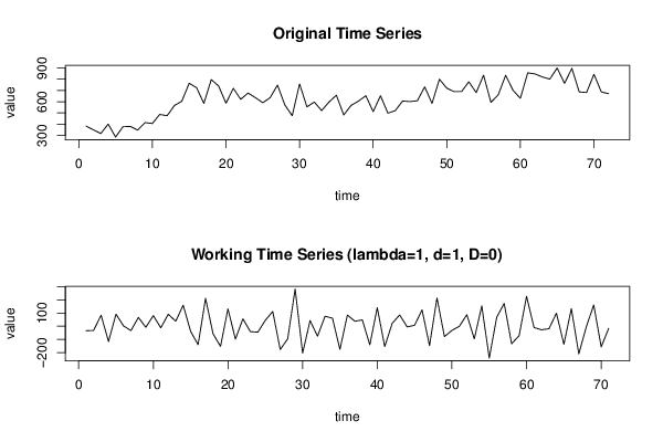
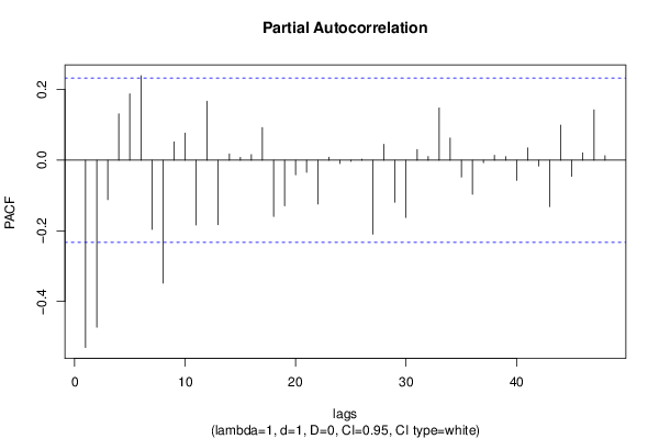
Title produced by software

(Partial) Autocorrelation Function

Date of computation

Tue, 06 Jan 2015 09:12:41 +0000

Cite this page as follows

Statistical Computations at FreeStatistics.org, Office for Research Development and Education, URL https://freestatistics.org/blog/index.php?v=date/2015/Jan/06/t1420535622ocobjyqcgm1xcfr.htm/, Retrieved Wed, 15 May 2024 13:15:56 +0000

Statistical Computations at FreeStatistics.org, Office for Research Development and Education, URL https://freestatistics.org/blog/index.php?pk=271990, Retrieved Wed, 15 May 2024 13:15:56 +0000

QR Codes:

Paste this QR Code to cite your computation.

Original text written by user:

IsPrivate?

No (this computation is public)

User-defined keywords

Estimated Impact

169

Family? (F = Feedback message, R = changed R code, M = changed R Module, P = changed Parameters, D = changed Data)

-     [Harrell-Davis Quantiles] [] [2015-01-05 16:01:40] [a8f6a7eeade7f89f597831d453788737]
-    D  [Harrell-Davis Quantiles] [] [2015-01-05 16:10:43] [a8f6a7eeade7f89f597831d453788737]
- RM        [(Partial) Autocorrelation Function] [] [2015-01-06 09:12:41] [12470bd120139be5e23c611c04d9c0dc] [Current]
- RM D        [Bootstrap Plot - Central Tendency] [] [2015-01-06 09:27:21] [a8f6a7eeade7f89f597831d453788737] 
- R             [Bootstrap Plot - Central Tendency] [] [2015-01-06 09:29:54] [a8f6a7eeade7f89f597831d453788737] 
-               [Bootstrap Plot - Central Tendency] [] [2015-01-06 09:33:28] [a8f6a7eeade7f89f597831d453788737] 
- RM D          [Blocked Bootstrap Plot - Central Tendency] [] [2015-01-06 10:19:09] [a8f6a7eeade7f89f597831d453788737] 
- RM D            [Variability] [] [2015-01-06 11:02:39] [a8f6a7eeade7f89f597831d453788737] 
- RM D            [Standard Deviation Plot] [] [2015-01-06 11:07:17] [a8f6a7eeade7f89f597831d453788737] 
- RM D            [Standard Deviation-Mean Plot] [] [2015-01-06 11:32:43] [a8f6a7eeade7f89f597831d453788737] 
- RM              [Variability] [] [2015-01-06 11:43:50] [a8f6a7eeade7f89f597831d453788737] 
- RM              [Standard Deviation Plot] [] [2015-01-06 11:48:58] [a8f6a7eeade7f89f597831d453788737] 
- RM              [Standard Deviation-Mean Plot] [] [2015-01-06 12:01:28] [a8f6a7eeade7f89f597831d453788737] 
- RM D            [Classical Decomposition] [] [2015-01-06 12:12:48] [a8f6a7eeade7f89f597831d453788737] 
- RM                [Exponential Smoothing] [] [2015-01-06 12:25:54] [a8f6a7eeade7f89f597831d453788737] 
- RM D              [Exponential Smoothing] [] [2015-01-06 12:34:40] [a8f6a7eeade7f89f597831d453788737] 

Feedback Forum

Post a new message

Dataseries X:

Download CSV

Histogram

Boxplots

Summary of computational transaction
Raw Input	view raw input (R code)
Raw Output	view raw output of R engine
Computing time	2 seconds
R Server	'Gwilym Jenkins' @ jenkins.wessa.net

\begin{tabular}{lllllllll}
\hline
Summary of computational transaction \tabularnewline
Raw Input & view raw input (R code)  \tabularnewline
Raw Output & view raw output of R engine  \tabularnewline
Computing time & 2 seconds \tabularnewline
R Server & 'Gwilym Jenkins' @ jenkins.wessa.net \tabularnewline
\hline
\end{tabular}
%Source: https://freestatistics.org/blog/index.php?pk=271990&T=0

[TABLE]
[ROW][C]Summary of computational transaction[/C][/ROW]
[ROW][C]Raw Input[/C][C]view raw input (R code) [/C][/ROW]
[ROW][C]Raw Output[/C][C]view raw output of R engine [/C][/ROW]
[ROW][C]Computing time[/C][C]2 seconds[/C][/ROW]
[ROW][C]R Server[/C][C]'Gwilym Jenkins' @ jenkins.wessa.net[/C][/ROW]
[/TABLE]
Source: https://freestatistics.org/blog/index.php?pk=271990&T=0

Globally Unique Identifier (entire table): ba.freestatistics.org/blog/index.php?pk=271990&T=0

As an alternative you can also use a QR Code:

The GUIDs for individual cells are displayed in the table below:

Summary of computational transaction
Raw Input	view raw input (R code)
Raw Output	view raw output of R engine
Computing time	2 seconds
R Server	'Gwilym Jenkins' @ jenkins.wessa.net

Autocorrelation Function
Time lag k	ACF(k)	T-STAT	P-value
1	-0.530378	-4.469	1.5e-05
2	-0.058493	-0.4929	0.311811
3	0.234196	1.9734	0.026173
4	-0.03108	-0.2619	0.397083
5	-0.05627	-0.4741	0.318428
6	0.092295	0.7777	0.219667
7	-0.205287	-1.7298	0.044008
8	0.10863	0.9153	0.181559
9	0.186594	1.5723	0.060167
10	-0.315015	-2.6544	0.0049
11	-0.012234	-0.1031	0.459093
12	0.373011	3.143	0.00122
13	-0.425884	-3.5886	0.000304
14	0.221641	1.8676	0.032974
15	-0.034706	-0.2924	0.385404
16	-0.07394	-0.623	0.26763
17	0.140764	1.1861	0.119769
18	-0.110611	-0.932	0.177241
19	-0.076023	-0.6406	0.261929
20	0.181852	1.5323	0.064945
21	-0.06948	-0.5854	0.280051
22	-0.200062	-1.6858	0.048117
23	0.261214	2.201	0.015493
24	-0.077979	-0.6571	0.256631
25	-0.143553	-1.2096	0.115222
26	0.213414	1.7983	0.038194
27	-0.23518	-1.9817	0.025695
28	0.211783	1.7845	0.039306
29	-0.07744	-0.6525	0.258087
30	-0.150122	-1.2649	0.105013
31	0.191409	1.6128	0.055608
32	0.021321	0.1797	0.428969
33	-0.129453	-1.0908	0.139527
34	0.024932	0.2101	0.417104
35	0.130804	1.1022	0.137053
36	-0.137796	-1.1611	0.124747
37	0.133944	1.1286	0.131426
38	-0.087943	-0.741	0.230563
39	-0.078444	-0.661	0.255381
40	0.276808	2.3324	0.011259
41	-0.216039	-1.8204	0.036458
42	-0.048303	-0.407	0.342613
43	0.15217	1.2822	0.101971
44	-0.028443	-0.2397	0.405642
45	-0.099096	-0.835	0.203259
46	0.092931	0.7831	0.2181
47	-0.005496	-0.0463	0.481596
48	-0.042067	-0.3545	0.36202

\begin{tabular}{lllllllll}
\hline
Autocorrelation Function \tabularnewline
Time lag k & ACF(k) & T-STAT & P-value \tabularnewline
1 & -0.530378 & -4.469 & 1.5e-05 \tabularnewline
2 & -0.058493 & -0.4929 & 0.311811 \tabularnewline
3 & 0.234196 & 1.9734 & 0.026173 \tabularnewline
4 & -0.03108 & -0.2619 & 0.397083 \tabularnewline
5 & -0.05627 & -0.4741 & 0.318428 \tabularnewline
6 & 0.092295 & 0.7777 & 0.219667 \tabularnewline
7 & -0.205287 & -1.7298 & 0.044008 \tabularnewline
8 & 0.10863 & 0.9153 & 0.181559 \tabularnewline
9 & 0.186594 & 1.5723 & 0.060167 \tabularnewline
10 & -0.315015 & -2.6544 & 0.0049 \tabularnewline
11 & -0.012234 & -0.1031 & 0.459093 \tabularnewline
12 & 0.373011 & 3.143 & 0.00122 \tabularnewline
13 & -0.425884 & -3.5886 & 0.000304 \tabularnewline
14 & 0.221641 & 1.8676 & 0.032974 \tabularnewline
15 & -0.034706 & -0.2924 & 0.385404 \tabularnewline
16 & -0.07394 & -0.623 & 0.26763 \tabularnewline
17 & 0.140764 & 1.1861 & 0.119769 \tabularnewline
18 & -0.110611 & -0.932 & 0.177241 \tabularnewline
19 & -0.076023 & -0.6406 & 0.261929 \tabularnewline
20 & 0.181852 & 1.5323 & 0.064945 \tabularnewline
21 & -0.06948 & -0.5854 & 0.280051 \tabularnewline
22 & -0.200062 & -1.6858 & 0.048117 \tabularnewline
23 & 0.261214 & 2.201 & 0.015493 \tabularnewline
24 & -0.077979 & -0.6571 & 0.256631 \tabularnewline
25 & -0.143553 & -1.2096 & 0.115222 \tabularnewline
26 & 0.213414 & 1.7983 & 0.038194 \tabularnewline
27 & -0.23518 & -1.9817 & 0.025695 \tabularnewline
28 & 0.211783 & 1.7845 & 0.039306 \tabularnewline
29 & -0.07744 & -0.6525 & 0.258087 \tabularnewline
30 & -0.150122 & -1.2649 & 0.105013 \tabularnewline
31 & 0.191409 & 1.6128 & 0.055608 \tabularnewline
32 & 0.021321 & 0.1797 & 0.428969 \tabularnewline
33 & -0.129453 & -1.0908 & 0.139527 \tabularnewline
34 & 0.024932 & 0.2101 & 0.417104 \tabularnewline
35 & 0.130804 & 1.1022 & 0.137053 \tabularnewline
36 & -0.137796 & -1.1611 & 0.124747 \tabularnewline
37 & 0.133944 & 1.1286 & 0.131426 \tabularnewline
38 & -0.087943 & -0.741 & 0.230563 \tabularnewline
39 & -0.078444 & -0.661 & 0.255381 \tabularnewline
40 & 0.276808 & 2.3324 & 0.011259 \tabularnewline
41 & -0.216039 & -1.8204 & 0.036458 \tabularnewline
42 & -0.048303 & -0.407 & 0.342613 \tabularnewline
43 & 0.15217 & 1.2822 & 0.101971 \tabularnewline
44 & -0.028443 & -0.2397 & 0.405642 \tabularnewline
45 & -0.099096 & -0.835 & 0.203259 \tabularnewline
46 & 0.092931 & 0.7831 & 0.2181 \tabularnewline
47 & -0.005496 & -0.0463 & 0.481596 \tabularnewline
48 & -0.042067 & -0.3545 & 0.36202 \tabularnewline
\hline
\end{tabular}
%Source: https://freestatistics.org/blog/index.php?pk=271990&T=1

[TABLE]
[ROW][C]Autocorrelation Function[/C][/ROW]
[ROW][C]Time lag k[/C][C]ACF(k)[/C][C]T-STAT[/C][C]P-value[/C][/ROW]
[ROW][C]1[/C][C]-0.530378[/C][C]-4.469[/C][C]1.5e-05[/C][/ROW]
[ROW][C]2[/C][C]-0.058493[/C][C]-0.4929[/C][C]0.311811[/C][/ROW]
[ROW][C]3[/C][C]0.234196[/C][C]1.9734[/C][C]0.026173[/C][/ROW]
[ROW][C]4[/C][C]-0.03108[/C][C]-0.2619[/C][C]0.397083[/C][/ROW]
[ROW][C]5[/C][C]-0.05627[/C][C]-0.4741[/C][C]0.318428[/C][/ROW]
[ROW][C]6[/C][C]0.092295[/C][C]0.7777[/C][C]0.219667[/C][/ROW]
[ROW][C]7[/C][C]-0.205287[/C][C]-1.7298[/C][C]0.044008[/C][/ROW]
[ROW][C]8[/C][C]0.10863[/C][C]0.9153[/C][C]0.181559[/C][/ROW]
[ROW][C]9[/C][C]0.186594[/C][C]1.5723[/C][C]0.060167[/C][/ROW]
[ROW][C]10[/C][C]-0.315015[/C][C]-2.6544[/C][C]0.0049[/C][/ROW]
[ROW][C]11[/C][C]-0.012234[/C][C]-0.1031[/C][C]0.459093[/C][/ROW]
[ROW][C]12[/C][C]0.373011[/C][C]3.143[/C][C]0.00122[/C][/ROW]
[ROW][C]13[/C][C]-0.425884[/C][C]-3.5886[/C][C]0.000304[/C][/ROW]
[ROW][C]14[/C][C]0.221641[/C][C]1.8676[/C][C]0.032974[/C][/ROW]
[ROW][C]15[/C][C]-0.034706[/C][C]-0.2924[/C][C]0.385404[/C][/ROW]
[ROW][C]16[/C][C]-0.07394[/C][C]-0.623[/C][C]0.26763[/C][/ROW]
[ROW][C]17[/C][C]0.140764[/C][C]1.1861[/C][C]0.119769[/C][/ROW]
[ROW][C]18[/C][C]-0.110611[/C][C]-0.932[/C][C]0.177241[/C][/ROW]
[ROW][C]19[/C][C]-0.076023[/C][C]-0.6406[/C][C]0.261929[/C][/ROW]
[ROW][C]20[/C][C]0.181852[/C][C]1.5323[/C][C]0.064945[/C][/ROW]
[ROW][C]21[/C][C]-0.06948[/C][C]-0.5854[/C][C]0.280051[/C][/ROW]
[ROW][C]22[/C][C]-0.200062[/C][C]-1.6858[/C][C]0.048117[/C][/ROW]
[ROW][C]23[/C][C]0.261214[/C][C]2.201[/C][C]0.015493[/C][/ROW]
[ROW][C]24[/C][C]-0.077979[/C][C]-0.6571[/C][C]0.256631[/C][/ROW]
[ROW][C]25[/C][C]-0.143553[/C][C]-1.2096[/C][C]0.115222[/C][/ROW]
[ROW][C]26[/C][C]0.213414[/C][C]1.7983[/C][C]0.038194[/C][/ROW]
[ROW][C]27[/C][C]-0.23518[/C][C]-1.9817[/C][C]0.025695[/C][/ROW]
[ROW][C]28[/C][C]0.211783[/C][C]1.7845[/C][C]0.039306[/C][/ROW]
[ROW][C]29[/C][C]-0.07744[/C][C]-0.6525[/C][C]0.258087[/C][/ROW]
[ROW][C]30[/C][C]-0.150122[/C][C]-1.2649[/C][C]0.105013[/C][/ROW]
[ROW][C]31[/C][C]0.191409[/C][C]1.6128[/C][C]0.055608[/C][/ROW]
[ROW][C]32[/C][C]0.021321[/C][C]0.1797[/C][C]0.428969[/C][/ROW]
[ROW][C]33[/C][C]-0.129453[/C][C]-1.0908[/C][C]0.139527[/C][/ROW]
[ROW][C]34[/C][C]0.024932[/C][C]0.2101[/C][C]0.417104[/C][/ROW]
[ROW][C]35[/C][C]0.130804[/C][C]1.1022[/C][C]0.137053[/C][/ROW]
[ROW][C]36[/C][C]-0.137796[/C][C]-1.1611[/C][C]0.124747[/C][/ROW]
[ROW][C]37[/C][C]0.133944[/C][C]1.1286[/C][C]0.131426[/C][/ROW]
[ROW][C]38[/C][C]-0.087943[/C][C]-0.741[/C][C]0.230563[/C][/ROW]
[ROW][C]39[/C][C]-0.078444[/C][C]-0.661[/C][C]0.255381[/C][/ROW]
[ROW][C]40[/C][C]0.276808[/C][C]2.3324[/C][C]0.011259[/C][/ROW]
[ROW][C]41[/C][C]-0.216039[/C][C]-1.8204[/C][C]0.036458[/C][/ROW]
[ROW][C]42[/C][C]-0.048303[/C][C]-0.407[/C][C]0.342613[/C][/ROW]
[ROW][C]43[/C][C]0.15217[/C][C]1.2822[/C][C]0.101971[/C][/ROW]
[ROW][C]44[/C][C]-0.028443[/C][C]-0.2397[/C][C]0.405642[/C][/ROW]
[ROW][C]45[/C][C]-0.099096[/C][C]-0.835[/C][C]0.203259[/C][/ROW]
[ROW][C]46[/C][C]0.092931[/C][C]0.7831[/C][C]0.2181[/C][/ROW]
[ROW][C]47[/C][C]-0.005496[/C][C]-0.0463[/C][C]0.481596[/C][/ROW]
[ROW][C]48[/C][C]-0.042067[/C][C]-0.3545[/C][C]0.36202[/C][/ROW]
[/TABLE]
Source: https://freestatistics.org/blog/index.php?pk=271990&T=1

Globally Unique Identifier (entire table): ba.freestatistics.org/blog/index.php?pk=271990&T=1

As an alternative you can also use a QR Code:

The GUIDs for individual cells are displayed in the table below:

Autocorrelation Function
Time lag k	ACF(k)	T-STAT	P-value
1	-0.530378	-4.469	1.5e-05
2	-0.058493	-0.4929	0.311811
3	0.234196	1.9734	0.026173
4	-0.03108	-0.2619	0.397083
5	-0.05627	-0.4741	0.318428
6	0.092295	0.7777	0.219667
7	-0.205287	-1.7298	0.044008
8	0.10863	0.9153	0.181559
9	0.186594	1.5723	0.060167
10	-0.315015	-2.6544	0.0049
11	-0.012234	-0.1031	0.459093
12	0.373011	3.143	0.00122
13	-0.425884	-3.5886	0.000304
14	0.221641	1.8676	0.032974
15	-0.034706	-0.2924	0.385404
16	-0.07394	-0.623	0.26763
17	0.140764	1.1861	0.119769
18	-0.110611	-0.932	0.177241
19	-0.076023	-0.6406	0.261929
20	0.181852	1.5323	0.064945
21	-0.06948	-0.5854	0.280051
22	-0.200062	-1.6858	0.048117
23	0.261214	2.201	0.015493
24	-0.077979	-0.6571	0.256631
25	-0.143553	-1.2096	0.115222
26	0.213414	1.7983	0.038194
27	-0.23518	-1.9817	0.025695
28	0.211783	1.7845	0.039306
29	-0.07744	-0.6525	0.258087
30	-0.150122	-1.2649	0.105013
31	0.191409	1.6128	0.055608
32	0.021321	0.1797	0.428969
33	-0.129453	-1.0908	0.139527
34	0.024932	0.2101	0.417104
35	0.130804	1.1022	0.137053
36	-0.137796	-1.1611	0.124747
37	0.133944	1.1286	0.131426
38	-0.087943	-0.741	0.230563
39	-0.078444	-0.661	0.255381
40	0.276808	2.3324	0.011259
41	-0.216039	-1.8204	0.036458
42	-0.048303	-0.407	0.342613
43	0.15217	1.2822	0.101971
44	-0.028443	-0.2397	0.405642
45	-0.099096	-0.835	0.203259
46	0.092931	0.7831	0.2181
47	-0.005496	-0.0463	0.481596
48	-0.042067	-0.3545	0.36202

Partial Autocorrelation Function
Time lag k	PACF(k)	T-STAT	P-value
1	-0.530378	-4.469	1.5e-05
2	-0.472791	-3.9838	8.1e-05
3	-0.111555	-0.94	0.175207
4	0.131177	1.1053	0.136377
5	0.187671	1.5813	0.059122
6	0.239277	2.0162	0.023782
7	-0.196111	-1.6525	0.051428
8	-0.348245	-2.9344	0.002249
9	0.052038	0.4385	0.331186
10	0.076833	0.6474	0.259727
11	-0.183504	-1.5462	0.063248
12	0.1669	1.4063	0.081994
13	-0.182804	-1.5403	0.063962
14	0.017553	0.1479	0.441418
15	0.008128	0.0685	0.472794
16	0.015838	0.1335	0.447105
17	0.092243	0.7773	0.219795
18	-0.159426	-1.3433	0.091719
19	-0.128907	-1.0862	0.140535
20	-0.041563	-0.3502	0.363605
21	-0.034513	-0.2908	0.386023
22	-0.123971	-1.0446	0.149876
23	0.00845	0.0712	0.471718
24	-0.009751	-0.0822	0.467374
25	-0.003294	-0.0278	0.488968
26	0.003075	0.0259	0.489701
27	-0.20959	-1.766	0.040844
28	0.045106	0.3801	0.352514
29	-0.119073	-1.0033	0.159555
30	-0.162053	-1.3655	0.088205
31	0.030371	0.2559	0.399381
32	0.010457	0.0881	0.465019
33	0.147809	1.2455	0.108529
34	0.062668	0.5281	0.299555
35	-0.047819	-0.4029	0.344105
36	-0.096732	-0.8151	0.208876
37	-0.007298	-0.0615	0.47557
38	0.014081	0.1186	0.452945
39	0.010233	0.0862	0.465764
40	-0.057148	-0.4815	0.315808
41	0.035071	0.2955	0.384232
42	-0.016514	-0.1392	0.444862
43	-0.131667	-1.1094	0.135492
44	0.099454	0.838	0.202417
45	-0.045762	-0.3856	0.350474
46	0.020624	0.1738	0.431265
47	0.142485	1.2006	0.116948
48	0.01267	0.1068	0.457641

\begin{tabular}{lllllllll}
\hline
Partial Autocorrelation Function \tabularnewline
Time lag k & PACF(k) & T-STAT & P-value \tabularnewline
1 & -0.530378 & -4.469 & 1.5e-05 \tabularnewline
2 & -0.472791 & -3.9838 & 8.1e-05 \tabularnewline
3 & -0.111555 & -0.94 & 0.175207 \tabularnewline
4 & 0.131177 & 1.1053 & 0.136377 \tabularnewline
5 & 0.187671 & 1.5813 & 0.059122 \tabularnewline
6 & 0.239277 & 2.0162 & 0.023782 \tabularnewline
7 & -0.196111 & -1.6525 & 0.051428 \tabularnewline
8 & -0.348245 & -2.9344 & 0.002249 \tabularnewline
9 & 0.052038 & 0.4385 & 0.331186 \tabularnewline
10 & 0.076833 & 0.6474 & 0.259727 \tabularnewline
11 & -0.183504 & -1.5462 & 0.063248 \tabularnewline
12 & 0.1669 & 1.4063 & 0.081994 \tabularnewline
13 & -0.182804 & -1.5403 & 0.063962 \tabularnewline
14 & 0.017553 & 0.1479 & 0.441418 \tabularnewline
15 & 0.008128 & 0.0685 & 0.472794 \tabularnewline
16 & 0.015838 & 0.1335 & 0.447105 \tabularnewline
17 & 0.092243 & 0.7773 & 0.219795 \tabularnewline
18 & -0.159426 & -1.3433 & 0.091719 \tabularnewline
19 & -0.128907 & -1.0862 & 0.140535 \tabularnewline
20 & -0.041563 & -0.3502 & 0.363605 \tabularnewline
21 & -0.034513 & -0.2908 & 0.386023 \tabularnewline
22 & -0.123971 & -1.0446 & 0.149876 \tabularnewline
23 & 0.00845 & 0.0712 & 0.471718 \tabularnewline
24 & -0.009751 & -0.0822 & 0.467374 \tabularnewline
25 & -0.003294 & -0.0278 & 0.488968 \tabularnewline
26 & 0.003075 & 0.0259 & 0.489701 \tabularnewline
27 & -0.20959 & -1.766 & 0.040844 \tabularnewline
28 & 0.045106 & 0.3801 & 0.352514 \tabularnewline
29 & -0.119073 & -1.0033 & 0.159555 \tabularnewline
30 & -0.162053 & -1.3655 & 0.088205 \tabularnewline
31 & 0.030371 & 0.2559 & 0.399381 \tabularnewline
32 & 0.010457 & 0.0881 & 0.465019 \tabularnewline
33 & 0.147809 & 1.2455 & 0.108529 \tabularnewline
34 & 0.062668 & 0.5281 & 0.299555 \tabularnewline
35 & -0.047819 & -0.4029 & 0.344105 \tabularnewline
36 & -0.096732 & -0.8151 & 0.208876 \tabularnewline
37 & -0.007298 & -0.0615 & 0.47557 \tabularnewline
38 & 0.014081 & 0.1186 & 0.452945 \tabularnewline
39 & 0.010233 & 0.0862 & 0.465764 \tabularnewline
40 & -0.057148 & -0.4815 & 0.315808 \tabularnewline
41 & 0.035071 & 0.2955 & 0.384232 \tabularnewline
42 & -0.016514 & -0.1392 & 0.444862 \tabularnewline
43 & -0.131667 & -1.1094 & 0.135492 \tabularnewline
44 & 0.099454 & 0.838 & 0.202417 \tabularnewline
45 & -0.045762 & -0.3856 & 0.350474 \tabularnewline
46 & 0.020624 & 0.1738 & 0.431265 \tabularnewline
47 & 0.142485 & 1.2006 & 0.116948 \tabularnewline
48 & 0.01267 & 0.1068 & 0.457641 \tabularnewline
\hline
\end{tabular}
%Source: https://freestatistics.org/blog/index.php?pk=271990&T=2

[TABLE]
[ROW][C]Partial Autocorrelation Function[/C][/ROW]
[ROW][C]Time lag k[/C][C]PACF(k)[/C][C]T-STAT[/C][C]P-value[/C][/ROW]
[ROW][C]1[/C][C]-0.530378[/C][C]-4.469[/C][C]1.5e-05[/C][/ROW]
[ROW][C]2[/C][C]-0.472791[/C][C]-3.9838[/C][C]8.1e-05[/C][/ROW]
[ROW][C]3[/C][C]-0.111555[/C][C]-0.94[/C][C]0.175207[/C][/ROW]
[ROW][C]4[/C][C]0.131177[/C][C]1.1053[/C][C]0.136377[/C][/ROW]
[ROW][C]5[/C][C]0.187671[/C][C]1.5813[/C][C]0.059122[/C][/ROW]
[ROW][C]6[/C][C]0.239277[/C][C]2.0162[/C][C]0.023782[/C][/ROW]
[ROW][C]7[/C][C]-0.196111[/C][C]-1.6525[/C][C]0.051428[/C][/ROW]
[ROW][C]8[/C][C]-0.348245[/C][C]-2.9344[/C][C]0.002249[/C][/ROW]
[ROW][C]9[/C][C]0.052038[/C][C]0.4385[/C][C]0.331186[/C][/ROW]
[ROW][C]10[/C][C]0.076833[/C][C]0.6474[/C][C]0.259727[/C][/ROW]
[ROW][C]11[/C][C]-0.183504[/C][C]-1.5462[/C][C]0.063248[/C][/ROW]
[ROW][C]12[/C][C]0.1669[/C][C]1.4063[/C][C]0.081994[/C][/ROW]
[ROW][C]13[/C][C]-0.182804[/C][C]-1.5403[/C][C]0.063962[/C][/ROW]
[ROW][C]14[/C][C]0.017553[/C][C]0.1479[/C][C]0.441418[/C][/ROW]
[ROW][C]15[/C][C]0.008128[/C][C]0.0685[/C][C]0.472794[/C][/ROW]
[ROW][C]16[/C][C]0.015838[/C][C]0.1335[/C][C]0.447105[/C][/ROW]
[ROW][C]17[/C][C]0.092243[/C][C]0.7773[/C][C]0.219795[/C][/ROW]
[ROW][C]18[/C][C]-0.159426[/C][C]-1.3433[/C][C]0.091719[/C][/ROW]
[ROW][C]19[/C][C]-0.128907[/C][C]-1.0862[/C][C]0.140535[/C][/ROW]
[ROW][C]20[/C][C]-0.041563[/C][C]-0.3502[/C][C]0.363605[/C][/ROW]
[ROW][C]21[/C][C]-0.034513[/C][C]-0.2908[/C][C]0.386023[/C][/ROW]
[ROW][C]22[/C][C]-0.123971[/C][C]-1.0446[/C][C]0.149876[/C][/ROW]
[ROW][C]23[/C][C]0.00845[/C][C]0.0712[/C][C]0.471718[/C][/ROW]
[ROW][C]24[/C][C]-0.009751[/C][C]-0.0822[/C][C]0.467374[/C][/ROW]
[ROW][C]25[/C][C]-0.003294[/C][C]-0.0278[/C][C]0.488968[/C][/ROW]
[ROW][C]26[/C][C]0.003075[/C][C]0.0259[/C][C]0.489701[/C][/ROW]
[ROW][C]27[/C][C]-0.20959[/C][C]-1.766[/C][C]0.040844[/C][/ROW]
[ROW][C]28[/C][C]0.045106[/C][C]0.3801[/C][C]0.352514[/C][/ROW]
[ROW][C]29[/C][C]-0.119073[/C][C]-1.0033[/C][C]0.159555[/C][/ROW]
[ROW][C]30[/C][C]-0.162053[/C][C]-1.3655[/C][C]0.088205[/C][/ROW]
[ROW][C]31[/C][C]0.030371[/C][C]0.2559[/C][C]0.399381[/C][/ROW]
[ROW][C]32[/C][C]0.010457[/C][C]0.0881[/C][C]0.465019[/C][/ROW]
[ROW][C]33[/C][C]0.147809[/C][C]1.2455[/C][C]0.108529[/C][/ROW]
[ROW][C]34[/C][C]0.062668[/C][C]0.5281[/C][C]0.299555[/C][/ROW]
[ROW][C]35[/C][C]-0.047819[/C][C]-0.4029[/C][C]0.344105[/C][/ROW]
[ROW][C]36[/C][C]-0.096732[/C][C]-0.8151[/C][C]0.208876[/C][/ROW]
[ROW][C]37[/C][C]-0.007298[/C][C]-0.0615[/C][C]0.47557[/C][/ROW]
[ROW][C]38[/C][C]0.014081[/C][C]0.1186[/C][C]0.452945[/C][/ROW]
[ROW][C]39[/C][C]0.010233[/C][C]0.0862[/C][C]0.465764[/C][/ROW]
[ROW][C]40[/C][C]-0.057148[/C][C]-0.4815[/C][C]0.315808[/C][/ROW]
[ROW][C]41[/C][C]0.035071[/C][C]0.2955[/C][C]0.384232[/C][/ROW]
[ROW][C]42[/C][C]-0.016514[/C][C]-0.1392[/C][C]0.444862[/C][/ROW]
[ROW][C]43[/C][C]-0.131667[/C][C]-1.1094[/C][C]0.135492[/C][/ROW]
[ROW][C]44[/C][C]0.099454[/C][C]0.838[/C][C]0.202417[/C][/ROW]
[ROW][C]45[/C][C]-0.045762[/C][C]-0.3856[/C][C]0.350474[/C][/ROW]
[ROW][C]46[/C][C]0.020624[/C][C]0.1738[/C][C]0.431265[/C][/ROW]
[ROW][C]47[/C][C]0.142485[/C][C]1.2006[/C][C]0.116948[/C][/ROW]
[ROW][C]48[/C][C]0.01267[/C][C]0.1068[/C][C]0.457641[/C][/ROW]
[/TABLE]
Source: https://freestatistics.org/blog/index.php?pk=271990&T=2

Globally Unique Identifier (entire table): ba.freestatistics.org/blog/index.php?pk=271990&T=2

As an alternative you can also use a QR Code:

The GUIDs for individual cells are displayed in the table below:

Partial Autocorrelation Function
Time lag k	PACF(k)	T-STAT	P-value
1	-0.530378	-4.469	1.5e-05
2	-0.472791	-3.9838	8.1e-05
3	-0.111555	-0.94	0.175207
4	0.131177	1.1053	0.136377
5	0.187671	1.5813	0.059122
6	0.239277	2.0162	0.023782
7	-0.196111	-1.6525	0.051428
8	-0.348245	-2.9344	0.002249
9	0.052038	0.4385	0.331186
10	0.076833	0.6474	0.259727
11	-0.183504	-1.5462	0.063248
12	0.1669	1.4063	0.081994
13	-0.182804	-1.5403	0.063962
14	0.017553	0.1479	0.441418
15	0.008128	0.0685	0.472794
16	0.015838	0.1335	0.447105
17	0.092243	0.7773	0.219795
18	-0.159426	-1.3433	0.091719
19	-0.128907	-1.0862	0.140535
20	-0.041563	-0.3502	0.363605
21	-0.034513	-0.2908	0.386023
22	-0.123971	-1.0446	0.149876
23	0.00845	0.0712	0.471718
24	-0.009751	-0.0822	0.467374
25	-0.003294	-0.0278	0.488968
26	0.003075	0.0259	0.489701
27	-0.20959	-1.766	0.040844
28	0.045106	0.3801	0.352514
29	-0.119073	-1.0033	0.159555
30	-0.162053	-1.3655	0.088205
31	0.030371	0.2559	0.399381
32	0.010457	0.0881	0.465019
33	0.147809	1.2455	0.108529
34	0.062668	0.5281	0.299555
35	-0.047819	-0.4029	0.344105
36	-0.096732	-0.8151	0.208876
37	-0.007298	-0.0615	0.47557
38	0.014081	0.1186	0.452945
39	0.010233	0.0862	0.465764
40	-0.057148	-0.4815	0.315808
41	0.035071	0.2955	0.384232
42	-0.016514	-0.1392	0.444862
43	-0.131667	-1.1094	0.135492
44	0.099454	0.838	0.202417
45	-0.045762	-0.3856	0.350474
46	0.020624	0.1738	0.431265
47	0.142485	1.2006	0.116948
48	0.01267	0.1068	0.457641

Figure 1

PNG link

Postscript link

PDF link

Figure 2

PNG link

Postscript link

PDF link

Figure 3

PNG link

Postscript link

PDF link

Parameters (Session):

par1 = 0.1 ; par2 = 0.9 ; par3 = 0.1 ;

Parameters (R input):

par1 = 48 ; par2 = 1 ; par3 = 1 ; par4 = 0 ; par5 = 12 ; par6 = White Noise ; par7 = 0.95 ; par8 = ;

R code (references can be found in the software module):

if (par1 == 'Default') {
par1 = 10*log10(length(x))
} else {
par1 <- as.numeric(par1)
}
par2 <- as.numeric(par2)
par3 <- as.numeric(par3)
par4 <- as.numeric(par4)
par5 <- as.numeric(par5)
if (par6 == 'White Noise') par6 <- 'white' else par6 <- 'ma'
par7 <- as.numeric(par7)
if (par8 != '') par8 <- as.numeric(par8)
ox <- x
if (par8 == '') {
if (par2 == 0) {
x <- log(x)
} else {
x <- (x ^ par2 - 1) / par2
}
} else {
x <- log(x,base=par8)
}
if (par3 > 0) x <- diff(x,lag=1,difference=par3)
if (par4 > 0) x <- diff(x,lag=par5,difference=par4)
bitmap(file='picts.png')
op <- par(mfrow=c(2,1))
plot(ox,type='l',main='Original Time Series',xlab='time',ylab='value')
if (par8=='') {
mytitle <- paste('Working Time Series (lambda=',par2,', d=',par3,', D=',par4,')',sep='')
mysub <- paste('(lambda=',par2,', d=',par3,', D=',par4,', CI=', par7, ', CI type=',par6,')',sep='')
} else {
mytitle <- paste('Working Time Series (base=',par8,', d=',par3,', D=',par4,')',sep='')
mysub <- paste('(base=',par8,', d=',par3,', D=',par4,', CI=', par7, ', CI type=',par6,')',sep='')
}
plot(x,type='l', main=mytitle,xlab='time',ylab='value')
par(op)
dev.off()
bitmap(file='pic1.png')
racf <- acf(x, par1, main='Autocorrelation', xlab='time lag', ylab='ACF', ci.type=par6, ci=par7, sub=mysub)
dev.off()
bitmap(file='pic2.png')
rpacf <- pacf(x,par1,main='Partial Autocorrelation',xlab='lags',ylab='PACF',sub=mysub)
dev.off()
(myacf <- c(racf$acf))
(mypacf <- c(rpacf$acf))
lengthx <- length(x)
sqrtn <- sqrt(lengthx)
load(file='createtable')
a<-table.start()
a<-table.row.start(a)
a<-table.element(a,'Autocorrelation Function',4,TRUE)
a<-table.row.end(a)
a<-table.row.start(a)
a<-table.element(a,'Time lag k',header=TRUE)
a<-table.element(a,hyperlink('basics.htm','ACF(k)','click here for more information about the Autocorrelation Function'),header=TRUE)
a<-table.element(a,'T-STAT',header=TRUE)
a<-table.element(a,'P-value',header=TRUE)
a<-table.row.end(a)
for (i in 2:(par1+1)) {
a<-table.row.start(a)
a<-table.element(a,i-1,header=TRUE)
a<-table.element(a,round(myacf[i],6))
mytstat <- myacf[i]*sqrtn
a<-table.element(a,round(mytstat,4))
a<-table.element(a,round(1-pt(abs(mytstat),lengthx),6))
a<-table.row.end(a)
}
a<-table.end(a)
table.save(a,file='mytable.tab')
a<-table.start()
a<-table.row.start(a)
a<-table.element(a,'Partial Autocorrelation Function',4,TRUE)
a<-table.row.end(a)
a<-table.row.start(a)
a<-table.element(a,'Time lag k',header=TRUE)
a<-table.element(a,hyperlink('basics.htm','PACF(k)','click here for more information about the Partial Autocorrelation Function'),header=TRUE)
a<-table.element(a,'T-STAT',header=TRUE)
a<-table.element(a,'P-value',header=TRUE)
a<-table.row.end(a)
for (i in 1:par1) {
a<-table.row.start(a)
a<-table.element(a,i,header=TRUE)
a<-table.element(a,round(mypacf[i],6))
mytstat <- mypacf[i]*sqrtn
a<-table.element(a,round(mytstat,4))
a<-table.element(a,round(1-pt(abs(mytstat),lengthx),6))
a<-table.row.end(a)
}
a<-table.end(a)
table.save(a,file='mytable1.tab')

Free Statistics

Description of Statistical Computation

Tree of Dependent Computations

Dataset

Tables (Output of Computation)

Figures (Output of Computation)

Input Parameters & R Code