Repository of Reproducible Computations

Free Statistics

of Irreproducible Research!

Author's title

Author

*The author of this computation has been verified*

R Software Module

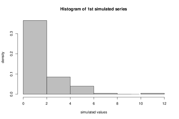
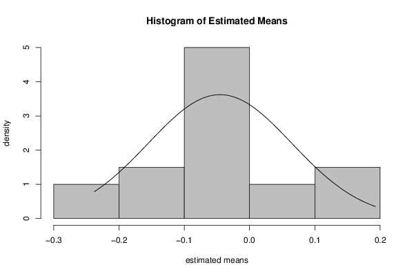
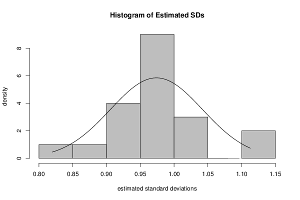
Title produced by software

Random Number Generator - Log-Normal Distribution

Date of computation

Wed, 23 Oct 2013 13:33:55 -0400

Cite this page as follows

Statistical Computations at FreeStatistics.org, Office for Research Development and Education, URL https://freestatistics.org/blog/index.php?v=date/2013/Oct/23/t138254964815vv5lgni8yfljo.htm/, Retrieved Sat, 27 Apr 2024 18:41:14 +0000

Statistical Computations at FreeStatistics.org, Office for Research Development and Education, URL https://freestatistics.org/blog/index.php?pk=219114, Retrieved Sat, 27 Apr 2024 18:41:14 +0000

QR Codes:

Paste this QR Code to cite your computation.

Original text written by user:

IsPrivate?

No (this computation is public)

User-defined keywords

Estimated Impact

Family? (F = Feedback message, R = changed R code, M = changed R Module, P = changed Parameters, D = changed Data)

-     [Notched Boxplots] [Academic Motivati...] [2010-10-12 12:51:42] [b98453cac15ba1066b407e146608df68]
- RM D  [Random Number Generator - Log-Normal Distribution] [] [2013-10-23 12:11:28] [d14f74cd5aff4c2cc0304b8517f6d549]
- R P     [Random Number Generator - Log-Normal Distribution] [] [2013-10-23 17:32:19] [156be4d2ddf8d2a15bc04845c69a1645]
-  M          [Random Number Generator - Log-Normal Distribution] [] [2013-10-23 17:33:55] [179dc240cf1f140d5d64fcae512f5803] [Current]

Feedback Forum

Post a new message

Summary of computational transaction
Raw Input	view raw input (R code)
Raw Output	view raw output of R engine
Computing time	3 seconds
R Server	'Gwilym Jenkins' @ jenkins.wessa.net

\begin{tabular}{lllllllll}
\hline
Summary of computational transaction \tabularnewline
Raw Input & view raw input (R code)  \tabularnewline
Raw Output & view raw output of R engine  \tabularnewline
Computing time & 3 seconds \tabularnewline
R Server & 'Gwilym Jenkins' @ jenkins.wessa.net \tabularnewline
\hline
\end{tabular}
%Source: https://freestatistics.org/blog/index.php?pk=219114&T=0

[TABLE]
[ROW][C]Summary of computational transaction[/C][/ROW]
[ROW][C]Raw Input[/C][C]view raw input (R code) [/C][/ROW]
[ROW][C]Raw Output[/C][C]view raw output of R engine [/C][/ROW]
[ROW][C]Computing time[/C][C]3 seconds[/C][/ROW]
[ROW][C]R Server[/C][C]'Gwilym Jenkins' @ jenkins.wessa.net[/C][/ROW]
[/TABLE]
Source: https://freestatistics.org/blog/index.php?pk=219114&T=0

Globally Unique Identifier (entire table): ba.freestatistics.org/blog/index.php?pk=219114&T=0

As an alternative you can also use a QR Code:

The GUIDs for individual cells are displayed in the table below:

Summary of computational transaction
Raw Input	view raw input (R code)
Raw Output	view raw output of R engine
Computing time	3 seconds
R Server	'Gwilym Jenkins' @ jenkins.wessa.net

Parameter	X1	X2	X3	X4	X5	X6	X7	X8	X9	X10
	(SD)	(SD)	(SD)	(SD)	(SD)	(SD)	(SD)	(SD)	(SD)	(SD)
# simulated values	100	100	100	100	100	100	100	100	100	100
true mean	0	0	0	0	0	0	0	0	0	0
true standard deviation	1	1	1	1	1	1	1	1	1	1
mean	0.04	-0.03	-0.09	-0.11	0	0.04	-0.24	-0.05	-0.09	-0.08
	0.1	0.11	0.09	0.1	0.11	0.1	0.1	0.1	0.1	0.1
standard deviation	1	1.11	0.94	1.03	1.11	0.98	1.04	0.97	0.96	0.97
	0.07	0.08	0.07	0.07	0.08	0.07	0.07	0.07	0.07	0.07

\begin{tabular}{lllllllll}
\hline
Parameter & X1 & X2 & X3 & X4 & X5 & X6 & X7 & X8 & X9 & X10 \tabularnewline
  & (SD) & (SD) & (SD) & (SD) & (SD) & (SD) & (SD) & (SD) & (SD) & (SD) \tabularnewline
# simulated values & 100 & 100 & 100 & 100 & 100 & 100 & 100 & 100 & 100 & 100 \tabularnewline
true mean & 0 & 0 & 0 & 0 & 0 & 0 & 0 & 0 & 0 & 0 \tabularnewline
true standard deviation & 1 & 1 & 1 & 1 & 1 & 1 & 1 & 1 & 1 & 1 \tabularnewline
mean & 0.04 & -0.03 & -0.09 & -0.11 & 0 & 0.04 & -0.24 & -0.05 & -0.09 & -0.08 \tabularnewline
  & 0.1 & 0.11 & 0.09 & 0.1 & 0.11 & 0.1 & 0.1 & 0.1 & 0.1 & 0.1 \tabularnewline
standard deviation & 1 & 1.11 & 0.94 & 1.03 & 1.11 & 0.98 & 1.04 & 0.97 & 0.96 & 0.97 \tabularnewline
  & 0.07 & 0.08 & 0.07 & 0.07 & 0.08 & 0.07 & 0.07 & 0.07 & 0.07 & 0.07 \tabularnewline
\hline
\end{tabular}
%Source: https://freestatistics.org/blog/index.php?pk=219114&T=1

[TABLE]
[ROW][C]Parameter[/C][C]X1[/C][C]X2[/C][C]X3[/C][C]X4[/C][C]X5[/C][C]X6[/C][C]X7[/C][C]X8[/C][C]X9[/C][C]X10[/C][/ROW]
[ROW][C] [/C][C](SD)[/C][C](SD)[/C][C](SD)[/C][C](SD)[/C][C](SD)[/C][C](SD)[/C][C](SD)[/C][C](SD)[/C][C](SD)[/C][C](SD)[/C][/ROW]
[ROW][C]# simulated values[/C][C]100[/C][C]100[/C][C]100[/C][C]100[/C][C]100[/C][C]100[/C][C]100[/C][C]100[/C][C]100[/C][C]100[/C][/ROW]
[ROW][C]true mean[/C][C]0[/C][C]0[/C][C]0[/C][C]0[/C][C]0[/C][C]0[/C][C]0[/C][C]0[/C][C]0[/C][C]0[/C][/ROW]
[ROW][C]true standard deviation[/C][C]1[/C][C]1[/C][C]1[/C][C]1[/C][C]1[/C][C]1[/C][C]1[/C][C]1[/C][C]1[/C][C]1[/C][/ROW]
[ROW][C]mean[/C][C]0.04[/C][C]-0.03[/C][C]-0.09[/C][C]-0.11[/C][C]0[/C][C]0.04[/C][C]-0.24[/C][C]-0.05[/C][C]-0.09[/C][C]-0.08[/C][/ROW]
[ROW][C] [/C][C]0.1[/C][C]0.11[/C][C]0.09[/C][C]0.1[/C][C]0.11[/C][C]0.1[/C][C]0.1[/C][C]0.1[/C][C]0.1[/C][C]0.1[/C][/ROW]
[ROW][C]standard deviation[/C][C]1[/C][C]1.11[/C][C]0.94[/C][C]1.03[/C][C]1.11[/C][C]0.98[/C][C]1.04[/C][C]0.97[/C][C]0.96[/C][C]0.97[/C][/ROW]
[ROW][C] [/C][C]0.07[/C][C]0.08[/C][C]0.07[/C][C]0.07[/C][C]0.08[/C][C]0.07[/C][C]0.07[/C][C]0.07[/C][C]0.07[/C][C]0.07[/C][/ROW]
[/TABLE]
Source: https://freestatistics.org/blog/index.php?pk=219114&T=1

Globally Unique Identifier (entire table): ba.freestatistics.org/blog/index.php?pk=219114&T=1

As an alternative you can also use a QR Code:

The GUIDs for individual cells are displayed in the table below:

Parameter	X1	X2	X3	X4	X5	X6	X7	X8	X9	X10
	(SD)	(SD)	(SD)	(SD)	(SD)	(SD)	(SD)	(SD)	(SD)	(SD)
# simulated values	100	100	100	100	100	100	100	100	100	100
true mean	0	0	0	0	0	0	0	0	0	0
true standard deviation	1	1	1	1	1	1	1	1	1	1
mean	0.04	-0.03	-0.09	-0.11	0	0.04	-0.24	-0.05	-0.09	-0.08
	0.1	0.11	0.09	0.1	0.11	0.1	0.1	0.1	0.1	0.1
standard deviation	1	1.11	0.94	1.03	1.11	0.98	1.04	0.97	0.96	0.97
	0.07	0.08	0.07	0.07	0.08	0.07	0.07	0.07	0.07	0.07

Figure 1

PNG link

Postscript link

PDF link

Figure 2

PNG link

Postscript link

PDF link

Figure 3

PNG link

Postscript link

PDF link

Parameters (Session):

par1 = 100 ; par2 = 0 ; par3 = 1 ; par4 = 8 ; par5 = N ; par6 = 0 ; par7 = 20 ;

Parameters (R input):

par1 = 100 ; par2 = 0 ; par3 = 1 ; par4 = 8 ; par5 = N ; par6 = 0 ; par7 = 20 ; par8 = ; par9 = ; par10 = ; par11 = ; par12 = ; par13 = ; par14 = ; par15 = ; par16 = ; par17 = ; par18 = ; par19 = ; par20 = ;

R code (references can be found in the software module):

library(MASS)
par1 <- as.numeric(par1)
par2 <- as.numeric(par2)
par2 <- round(par2,2) #rounded (we want to be able to display 10 columns)
par3 <- as.numeric(par3)
par3 <- round(par3,2) #rounded (we want to be able to display 10 columns)
par4 <- as.numeric(par4)
if (par6 == '0') par6 = 'Sturges' else par6 <- as.numeric(par6)
par7 <- as.numeric(par7)
x <- array(NA,dim=c(par7,par1))
rest.mean <- array(NA,dim=c(par7))
rest.sd <- array(NA,dim=c(par7))
rsd.mean <- array(NA,dim=c(par7))
rsd.sd <- array(NA,dim=c(par7))
for (i in 1:par7)
{
x[i,] <- rlnorm(par1,par2,par3)
x[i,] <- as.ts(x[i,]) #otherwise the fitdistr function does not work properly
dum <- fitdistr(x[i,],'log-normal')
rest.mean[i] <- dum$estimate[1]
rest.sd[i] <- dum$estimate[2]
rsd.mean[i] <- dum$sd[1]
rsd.sd[i] <- dum$sd[2]
}
nc <- par7
if (nc > 10) nc = 10
if (par5 == 'Y')
{
load(file='createtable')
a<-table.start()
a<-table.row.start(a)
a<-table.element(a,'Index',1,TRUE)
for (j in 1:nc)
{
a<-table.element(a,paste('X',j),1,TRUE)
}
a<-table.row.end(a)
if (nc < par7)
{
a<-table.row.start(a)
a<-table.element(a,'Note: only the first 10 series are displayed',nc+1,TRUE)
a<-table.row.end(a)
}
for (i in 1:par1)
{
a<-table.row.start(a)
a<-table.element(a,i,header=TRUE)
for (j in 1:nc)
{
a<-table.element(a,round(x[j,i],2))
}
a<-table.row.end(a)
}
a<-table.end(a)
table.save(a,file='mytable1.tab')
}
load(file='createtable')
a<-table.start()
a<-table.row.start(a)
a<-table.element(a,'Parameter',1,TRUE)
for (j in 1:nc)
{
a<-table.element(a,paste('X',j,sep=''),1,TRUE)
}
a<-table.row.end(a)
a<-table.row.start(a)
a<-table.element(a,' ',1,TRUE)
for (j in 1:nc)
{
a<-table.element(a,'(SD)',1,TRUE)
}
a<-table.row.end(a)
a<-table.row.start(a)
a<-table.element(a,'# simulated values',header=TRUE)
for (j in 1:nc)
{
a<-table.element(a,par1)
}
a<-table.row.end(a)
a<-table.row.start(a)
a<-table.element(a,'true mean',header=TRUE)
for (j in 1:nc)
{
a<-table.element(a,par2)
}
a<-table.row.end(a)
a<-table.row.start(a)
a<-table.element(a,'true standard deviation',header=TRUE)
for (j in 1:nc)
{
a<-table.element(a,par3)
}
a<-table.row.end(a)
a<-table.row.start(a)
a<-table.element(a,'mean',header=TRUE)
for (j in 1:nc)
{
a<-table.element(a,round(rest.mean[j],2))
}
a<-table.row.end(a)
a<-table.row.start(a)
a<-table.element(a,' ',header=TRUE)
for (j in 1:nc)
{
a<-table.element(a,round(rsd.mean[j],2))
}
a<-table.row.end(a)
a<-table.row.start(a)
a<-table.element(a,'standard deviation',header=TRUE)
for (j in 1:nc)
{
a<-table.element(a,round(rest.sd[j],2))
}
a<-table.row.end(a)
a<-table.row.start(a)
a<-table.element(a,' ',header=TRUE)
for (j in 1:nc)
{
a<-table.element(a,round(rsd.sd[j],2))
}
a<-table.row.end(a)
a<-table.end(a)
table.save(a,file='mytable.tab')
bitmap(file='test0.png')
myhist<-hist(x[1,],col=par4,breaks=par6,main='Histogram of 1st simulated series',ylab='density',xlab='simulated values',freq=F)
dev.off()
bitmap(file='test1.png')
myhist<-hist(rest.mean[],col=par4,breaks=par6,main='Histogram of Estimated Means',ylab='density',xlab='estimated means',freq=F)
x <- rest.mean[]
dummean <- mean(x)
dumsd <- sd(x)
curve(1/(dumsd*sqrt(2*pi))*exp(-1/2*((x-dummean)/dumsd)^2),min(x),max(x),add=T)
dev.off()
bitmap(file='test2.png')
myhist<-hist(rest.sd[],col=par4,breaks=par6,main='Histogram of Estimated SDs',ylab='density',xlab='estimated standard deviations',freq=F)
x <- rest.sd[]
dummean <- mean(x)
dumsd <- sd(x)
curve(1/(dumsd*sqrt(2*pi))*exp(-1/2*((x-dummean)/dumsd)^2),min(x),max(x),add=T)
dev.off()

Free Statistics

Description of Statistical Computation

Tree of Dependent Computations

Dataset

Tables (Output of Computation)

Figures (Output of Computation)

Input Parameters & R Code