Free Statistics

of Irreproducible Research!

Author's title

Author*The author of this computation has been verified*
R Software Modulerwasp_rnglnorm.wasp
Title produced by softwareRandom Number Generator - Log-Normal Distribution
Date of computationWed, 23 Oct 2013 10:03:04 -0400
Cite this page as followsStatistical Computations at FreeStatistics.org, Office for Research Development and Education, URL https://freestatistics.org/blog/index.php?v=date/2013/Oct/23/t1382537008an9413d4s94z6dh.htm/, Retrieved Sat, 27 Apr 2024 16:45:02 +0000
Statistical Computations at FreeStatistics.org, Office for Research Development and Education, URL https://freestatistics.org/blog/index.php?pk=218955, Retrieved Sat, 27 Apr 2024 16:45:02 +0000
QR Codes:

Original text written by user:
IsPrivate?No (this computation is public)
User-defined keywords
Estimated Impact75
Family? (F = Feedback message, R = changed R code, M = changed R Module, P = changed Parameters, D = changed Data)
-       [Random Number Generator - Log-Normal Distribution] [workshop 3 task 7] [2013-10-23 14:03:04] [249761a82d67c41cbe9b5c486860cdc6] [Current]
- R P     [Random Number Generator - Log-Normal Distribution] [workshop 3 task 7.2] [2013-10-23 14:04:05] [4e6b221caf797a012ce5465db674848b]
-   P       [Random Number Generator - Log-Normal Distribution] [workshop 3 task 7.3] [2013-10-23 14:07:29] [4e6b221caf797a012ce5465db674848b]
Feedback Forum

Post a new message


Summary of computational transaction
Raw Inputview raw input (R code)
Raw Outputview raw output of R engine
Computing time2 seconds
R Server'Gertrude Mary Cox' @ cox.wessa.net

\begin{tabular}{lllllllll}
\hline
Summary of computational transaction \tabularnewline
Raw Input & view raw input (R code)  \tabularnewline
Raw Output & view raw output of R engine  \tabularnewline
Computing time & 2 seconds \tabularnewline
R Server & 'Gertrude Mary Cox' @ cox.wessa.net \tabularnewline
\hline
\end{tabular}
%Source: https://freestatistics.org/blog/index.php?pk=218955&T=0

[TABLE]
[ROW][C]Summary of computational transaction[/C][/ROW]
[ROW][C]Raw Input[/C][C]view raw input (R code) [/C][/ROW]
[ROW][C]Raw Output[/C][C]view raw output of R engine [/C][/ROW]
[ROW][C]Computing time[/C][C]2 seconds[/C][/ROW]
[ROW][C]R Server[/C][C]'Gertrude Mary Cox' @ cox.wessa.net[/C][/ROW]
[/TABLE]
Source: https://freestatistics.org/blog/index.php?pk=218955&T=0

Globally Unique Identifier (entire table): ba.freestatistics.org/blog/index.php?pk=218955&T=0

As an alternative you can also use a QR Code:  

The GUIDs for individual cells are displayed in the table below:

Summary of computational transaction
Raw Inputview raw input (R code)
Raw Outputview raw output of R engine
Computing time2 seconds
R Server'Gertrude Mary Cox' @ cox.wessa.net


ParameterX1X2X3X4X5X6X7X8X9X10
(SD)(SD)(SD)(SD)(SD)(SD)(SD)(SD)(SD)(SD)
# simulated values100100100100100100100100100100
true mean0000000000
true standard deviation1111111111
mean0.06-0.03-0.13-0.090-0.130.180-0.03-0.13
0.090.090.10.10.10.10.10.110.10.09
standard deviation0.930.9110.961.030.960.971.10.960.94
0.070.060.070.070.070.070.070.080.070.07

\begin{tabular}{lllllllll}
\hline
Parameter & X1 & X2 & X3 & X4 & X5 & X6 & X7 & X8 & X9 & X10 \tabularnewline
  & (SD) & (SD) & (SD) & (SD) & (SD) & (SD) & (SD) & (SD) & (SD) & (SD) \tabularnewline
# simulated values & 100 & 100 & 100 & 100 & 100 & 100 & 100 & 100 & 100 & 100 \tabularnewline
true mean & 0 & 0 & 0 & 0 & 0 & 0 & 0 & 0 & 0 & 0 \tabularnewline
true standard deviation & 1 & 1 & 1 & 1 & 1 & 1 & 1 & 1 & 1 & 1 \tabularnewline
mean & 0.06 & -0.03 & -0.13 & -0.09 & 0 & -0.13 & 0.18 & 0 & -0.03 & -0.13 \tabularnewline
  & 0.09 & 0.09 & 0.1 & 0.1 & 0.1 & 0.1 & 0.1 & 0.11 & 0.1 & 0.09 \tabularnewline
standard deviation & 0.93 & 0.91 & 1 & 0.96 & 1.03 & 0.96 & 0.97 & 1.1 & 0.96 & 0.94 \tabularnewline
  & 0.07 & 0.06 & 0.07 & 0.07 & 0.07 & 0.07 & 0.07 & 0.08 & 0.07 & 0.07 \tabularnewline
\hline
\end{tabular}
%Source: https://freestatistics.org/blog/index.php?pk=218955&T=1

[TABLE]
[ROW][C]Parameter[/C][C]X1[/C][C]X2[/C][C]X3[/C][C]X4[/C][C]X5[/C][C]X6[/C][C]X7[/C][C]X8[/C][C]X9[/C][C]X10[/C][/ROW]
[ROW][C] [/C][C](SD)[/C][C](SD)[/C][C](SD)[/C][C](SD)[/C][C](SD)[/C][C](SD)[/C][C](SD)[/C][C](SD)[/C][C](SD)[/C][C](SD)[/C][/ROW]
[ROW][C]# simulated values[/C][C]100[/C][C]100[/C][C]100[/C][C]100[/C][C]100[/C][C]100[/C][C]100[/C][C]100[/C][C]100[/C][C]100[/C][/ROW]
[ROW][C]true mean[/C][C]0[/C][C]0[/C][C]0[/C][C]0[/C][C]0[/C][C]0[/C][C]0[/C][C]0[/C][C]0[/C][C]0[/C][/ROW]
[ROW][C]true standard deviation[/C][C]1[/C][C]1[/C][C]1[/C][C]1[/C][C]1[/C][C]1[/C][C]1[/C][C]1[/C][C]1[/C][C]1[/C][/ROW]
[ROW][C]mean[/C][C]0.06[/C][C]-0.03[/C][C]-0.13[/C][C]-0.09[/C][C]0[/C][C]-0.13[/C][C]0.18[/C][C]0[/C][C]-0.03[/C][C]-0.13[/C][/ROW]
[ROW][C] [/C][C]0.09[/C][C]0.09[/C][C]0.1[/C][C]0.1[/C][C]0.1[/C][C]0.1[/C][C]0.1[/C][C]0.11[/C][C]0.1[/C][C]0.09[/C][/ROW]
[ROW][C]standard deviation[/C][C]0.93[/C][C]0.91[/C][C]1[/C][C]0.96[/C][C]1.03[/C][C]0.96[/C][C]0.97[/C][C]1.1[/C][C]0.96[/C][C]0.94[/C][/ROW]
[ROW][C] [/C][C]0.07[/C][C]0.06[/C][C]0.07[/C][C]0.07[/C][C]0.07[/C][C]0.07[/C][C]0.07[/C][C]0.08[/C][C]0.07[/C][C]0.07[/C][/ROW]
[/TABLE]
Source: https://freestatistics.org/blog/index.php?pk=218955&T=1

Globally Unique Identifier (entire table): ba.freestatistics.org/blog/index.php?pk=218955&T=1

As an alternative you can also use a QR Code:  

The GUIDs for individual cells are displayed in the table below:

ParameterX1X2X3X4X5X6X7X8X9X10
(SD)(SD)(SD)(SD)(SD)(SD)(SD)(SD)(SD)(SD)
# simulated values100100100100100100100100100100
true mean0000000000
true standard deviation1111111111
mean0.06-0.03-0.13-0.090-0.130.180-0.03-0.13
0.090.090.10.10.10.10.10.110.10.09
standard deviation0.930.9110.961.030.960.971.10.960.94
0.070.060.070.070.070.070.070.080.070.07


Parameters (Session):
par1 = 100 ; par2 = 0 ; par3 = 1 ; par4 = 8 ; par5 = N ; par6 = 0 ; par7 = 20 ;
Parameters (R input):
par1 = 100 ; par2 = 0 ; par3 = 1 ; par4 = 8 ; par5 = N ; par6 = 0 ; par7 = 20 ;
R code (references can be found in the software module):
library(MASS)
par1 <- as.numeric(par1)
par2 <- as.numeric(par2)
par2 <- round(par2,2) #rounded (we want to be able to display 10 columns)
par3 <- as.numeric(par3)
par3 <- round(par3,2) #rounded (we want to be able to display 10 columns)
par4 <- as.numeric(par4)
if (par6 == '0') par6 = 'Sturges' else par6 <- as.numeric(par6)
par7 <- as.numeric(par7)
x <- array(NA,dim=c(par7,par1))
rest.mean <- array(NA,dim=c(par7))
rest.sd <- array(NA,dim=c(par7))
rsd.mean <- array(NA,dim=c(par7))
rsd.sd <- array(NA,dim=c(par7))
for (i in 1:par7)
{
x[i,] <- rlnorm(par1,par2,par3)
x[i,] <- as.ts(x[i,]) #otherwise the fitdistr function does not work properly
dum <- fitdistr(x[i,],'log-normal')
rest.mean[i] <- dum$estimate[1]
rest.sd[i] <- dum$estimate[2]
rsd.mean[i] <- dum$sd[1]
rsd.sd[i] <- dum$sd[2]
}
nc <- par7
if (nc > 10) nc = 10
if (par5 == 'Y')
{
load(file='createtable')
a<-table.start()
a<-table.row.start(a)
a<-table.element(a,'Index',1,TRUE)
for (j in 1:nc)
{
a<-table.element(a,paste('X',j),1,TRUE)
}
a<-table.row.end(a)
if (nc < par7)
{
a<-table.row.start(a)
a<-table.element(a,'Note: only the first 10 series are displayed',nc+1,TRUE)
a<-table.row.end(a)
}
for (i in 1:par1)
{
a<-table.row.start(a)
a<-table.element(a,i,header=TRUE)
for (j in 1:nc)
{
a<-table.element(a,round(x[j,i],2))
}
a<-table.row.end(a)
}
a<-table.end(a)
table.save(a,file='mytable1.tab')
}
load(file='createtable')
a<-table.start()
a<-table.row.start(a)
a<-table.element(a,'Parameter',1,TRUE)
for (j in 1:nc)
{
a<-table.element(a,paste('X',j,sep=''),1,TRUE)
}
a<-table.row.end(a)
a<-table.row.start(a)
a<-table.element(a,' ',1,TRUE)
for (j in 1:nc)
{
a<-table.element(a,'(SD)',1,TRUE)
}
a<-table.row.end(a)
a<-table.row.start(a)
a<-table.element(a,'# simulated values',header=TRUE)
for (j in 1:nc)
{
a<-table.element(a,par1)
}
a<-table.row.end(a)
a<-table.row.start(a)
a<-table.element(a,'true mean',header=TRUE)
for (j in 1:nc)
{
a<-table.element(a,par2)
}
a<-table.row.end(a)
a<-table.row.start(a)
a<-table.element(a,'true standard deviation',header=TRUE)
for (j in 1:nc)
{
a<-table.element(a,par3)
}
a<-table.row.end(a)
a<-table.row.start(a)
a<-table.element(a,'mean',header=TRUE)
for (j in 1:nc)
{
a<-table.element(a,round(rest.mean[j],2))
}
a<-table.row.end(a)
a<-table.row.start(a)
a<-table.element(a,' ',header=TRUE)
for (j in 1:nc)
{
a<-table.element(a,round(rsd.mean[j],2))
}
a<-table.row.end(a)
a<-table.row.start(a)
a<-table.element(a,'standard deviation',header=TRUE)
for (j in 1:nc)
{
a<-table.element(a,round(rest.sd[j],2))
}
a<-table.row.end(a)
a<-table.row.start(a)
a<-table.element(a,' ',header=TRUE)
for (j in 1:nc)
{
a<-table.element(a,round(rsd.sd[j],2))
}
a<-table.row.end(a)
a<-table.end(a)
table.save(a,file='mytable.tab')
bitmap(file='test0.png')
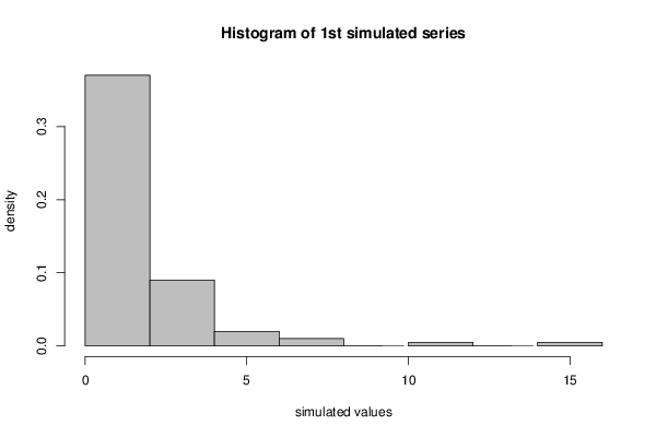
myhist<-hist(x[1,],col=par4,breaks=par6,main='Histogram of 1st simulated series',ylab='density',xlab='simulated values',freq=F)
dev.off()
bitmap(file='test1.png')
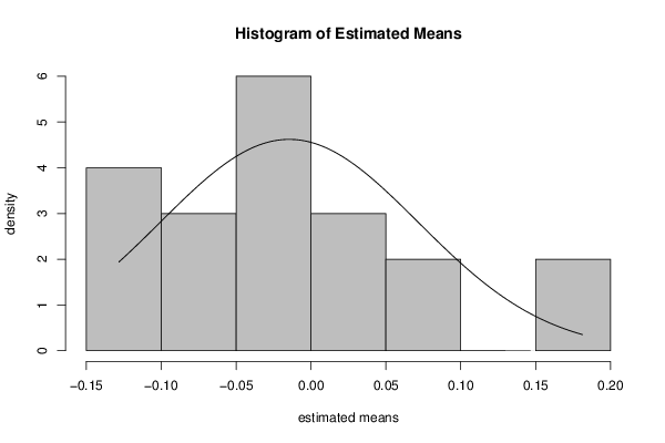
myhist<-hist(rest.mean[],col=par4,breaks=par6,main='Histogram of Estimated Means',ylab='density',xlab='estimated means',freq=F)
x <- rest.mean[]
dummean <- mean(x)
dumsd <- sd(x)
curve(1/(dumsd*sqrt(2*pi))*exp(-1/2*((x-dummean)/dumsd)^2),min(x),max(x),add=T)
dev.off()
bitmap(file='test2.png')
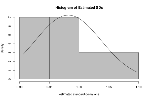
myhist<-hist(rest.sd[],col=par4,breaks=par6,main='Histogram of Estimated SDs',ylab='density',xlab='estimated standard deviations',freq=F)
x <- rest.sd[]
dummean <- mean(x)
dumsd <- sd(x)
curve(1/(dumsd*sqrt(2*pi))*exp(-1/2*((x-dummean)/dumsd)^2),min(x),max(x),add=T)
dev.off()