Free Statistics
of Irreproducible Research!
Description of Statistical Computation | |||||||||||||||||||||
|---|---|---|---|---|---|---|---|---|---|---|---|---|---|---|---|---|---|---|---|---|---|
| Author's title | |||||||||||||||||||||
| Author | *Unverified author* | ||||||||||||||||||||
| R Software Module | rwasp_meanplot.wasp | ||||||||||||||||||||
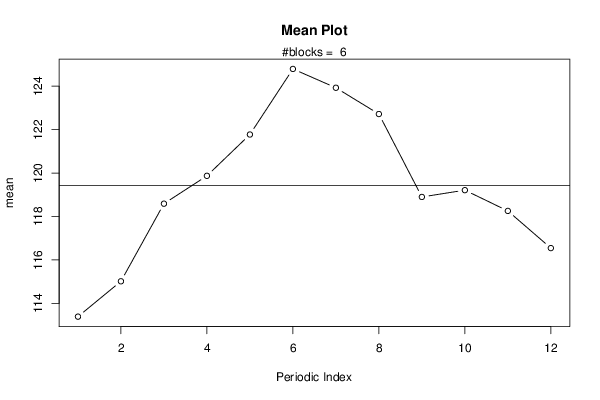
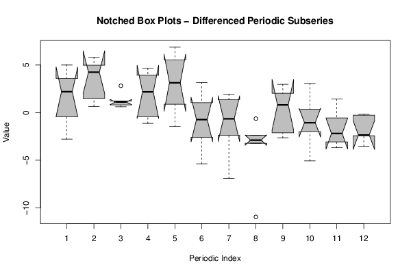
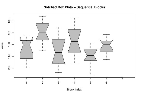
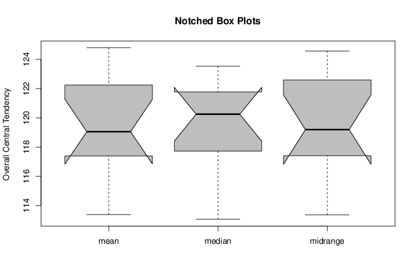
| Title produced by software | Mean Plot | ||||||||||||||||||||
| Date of computation | Sat, 19 Oct 2013 13:14:47 -0400 | ||||||||||||||||||||
| Cite this page as follows | Statistical Computations at FreeStatistics.org, Office for Research Development and Education, URL https://freestatistics.org/blog/index.php?v=date/2013/Oct/19/t1382202898w45ktm5ennu718v.htm/, Retrieved Mon, 29 Apr 2024 21:57:50 +0000 | ||||||||||||||||||||
| Statistical Computations at FreeStatistics.org, Office for Research Development and Education, URL https://freestatistics.org/blog/index.php?pk=216839, Retrieved Mon, 29 Apr 2024 21:57:50 +0000 | |||||||||||||||||||||
| QR Codes: | |||||||||||||||||||||
|
| |||||||||||||||||||||
| Original text written by user: | |||||||||||||||||||||
| IsPrivate? | No (this computation is public) | ||||||||||||||||||||
| User-defined keywords | |||||||||||||||||||||
| Estimated Impact | 62 | ||||||||||||||||||||
Tree of Dependent Computations | |||||||||||||||||||||
| Family? (F = Feedback message, R = changed R code, M = changed R Module, P = changed Parameters, D = changed Data) | |||||||||||||||||||||
| - [Mean Plot] [] [2013-10-19 17:14:47] [982f1398cb3cf8a81b54f385eadfb987] [Current] | |||||||||||||||||||||
| Feedback Forum | |||||||||||||||||||||
Post a new message | |||||||||||||||||||||
Dataset | |||||||||||||||||||||
| Dataseries X: | |||||||||||||||||||||
110,12 112,28 113,77 114,38 119,06 119,94 120,98 122,33 121,7 123,73 121,73 119,75 117,4 120,99 125,18 126,41 129,38 131,93 129,34 128,58 125,37 123,25 122,78 120,37 116,83 116,39 120,69 123,51 127,43 125,99 120,62 113,71 110,79 108,15 111,22 112,65 112,47 117,48 122,46 123,46 122,33 129,2 129,22 131,17 120,22 120,38 115,32 112,25 109,83 107,05 112,87 113,68 115,08 120,61 119,14 118,63 115,78 117,26 117,61 113,92 113,65 115,89 116,55 117,78 117,36 121,09 124,26 121,88 119,52 122,49 120,86 120,31 | |||||||||||||||||||||
Tables (Output of Computation) | |||||||||||||||||||||
| |||||||||||||||||||||
Figures (Output of Computation) | |||||||||||||||||||||
Input Parameters & R Code | |||||||||||||||||||||
| Parameters (Session): | |||||||||||||||||||||
| par1 = 12 ; | |||||||||||||||||||||
| Parameters (R input): | |||||||||||||||||||||
| par1 = 12 ; | |||||||||||||||||||||
| R code (references can be found in the software module): | |||||||||||||||||||||
par1 <- as.numeric(par1) | |||||||||||||||||||||