Repository of Reproducible Computations

Free Statistics

of Irreproducible Research!

Author's title

Author

*Unverified author*

R Software Module

rwasp_autocorrelation.wasp

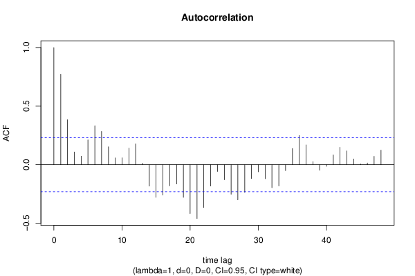
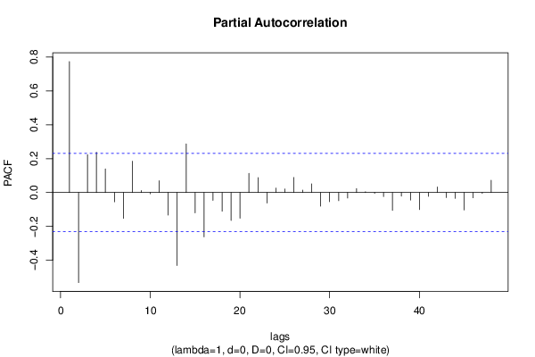
Title produced by software

(Partial) Autocorrelation Function

Date of computation

Sun, 26 May 2013 19:26:36 -0400

Cite this page as follows

Statistical Computations at FreeStatistics.org, Office for Research Development and Education, URL https://freestatistics.org/blog/index.php?v=date/2013/May/26/t1369610812rejdo50xisrdps1.htm/, Retrieved Mon, 29 Apr 2024 08:20:29 +0000

Statistical Computations at FreeStatistics.org, Office for Research Development and Education, URL https://freestatistics.org/blog/index.php?pk=210683, Retrieved Mon, 29 Apr 2024 08:20:29 +0000

QR Codes:

Paste this QR Code to cite your computation.

Original text written by user:

IsPrivate?

No (this computation is public)

User-defined keywords

Estimated Impact

100

Family? (F = Feedback message, R = changed R code, M = changed R Module, P = changed Parameters, D = changed Data)

-     [Mean Plot] [Inschrijvingen ni...] [2012-03-09 13:44:23] [dd1db122e2fe6bd517fcf7008a48ce3e]
- RMP   [(Partial) Autocorrelation Function] [] [2013-05-26 23:17:52] [f974b105a61ab974a820d469d59cfaf7]
-    D      [(Partial) Autocorrelation Function] [] [2013-05-26 23:26:36] [8f84a338303fe8d74ac0d8ad91c8b331] [Current]
- R PD        [(Partial) Autocorrelation Function] [] [2013-05-26 23:28:31] [f974b105a61ab974a820d469d59cfaf7] 
- RMPD        [Variability] [] [2013-05-27 00:21:49] [f974b105a61ab974a820d469d59cfaf7] 
- RMPD        [Standard Deviation Plot] [] [2013-05-27 00:25:06] [f974b105a61ab974a820d469d59cfaf7] 
- RMPD        [Standard Deviation-Mean Plot] [] [2013-05-27 00:32:33] [f974b105a61ab974a820d469d59cfaf7] 
- RMP         [Variability] [] [2013-05-27 00:36:53] [f974b105a61ab974a820d469d59cfaf7] 
- RMPD        [Standard Deviation Plot] [] [2013-05-27 00:39:33] [f974b105a61ab974a820d469d59cfaf7] 
- RMPD        [Standard Deviation-Mean Plot] [] [2013-05-27 00:44:15] [f974b105a61ab974a820d469d59cfaf7] 
- RMPD        [Classical Decomposition] [] [2013-05-27 00:48:49] [f974b105a61ab974a820d469d59cfaf7] 
- R             [Classical Decomposition] [] [2013-05-27 00:54:58] [f974b105a61ab974a820d469d59cfaf7] 
-    D          [Classical Decomposition] [] [2013-05-27 01:03:15] [f974b105a61ab974a820d469d59cfaf7] 
- RM            [Exponential Smoothing] [] [2013-05-27 01:07:25] [2f0f353a58a70fd7baf0f5141860d820] 
- RM D          [Exponential Smoothing] [] [2013-05-27 01:10:03] [2f0f353a58a70fd7baf0f5141860d820] 

Feedback Forum

Post a new message

Dataseries X:

Download CSV

Histogram

Boxplots

Summary of computational transaction
Raw Input	view raw input (R code)
Raw Output	view raw output of R engine
Computing time	3 seconds
R Server	'Herman Ole Andreas Wold' @ wold.wessa.net

\begin{tabular}{lllllllll}
\hline
Summary of computational transaction \tabularnewline
Raw Input & view raw input (R code)  \tabularnewline
Raw Output & view raw output of R engine  \tabularnewline
Computing time & 3 seconds \tabularnewline
R Server & 'Herman Ole Andreas Wold' @ wold.wessa.net \tabularnewline
\hline
\end{tabular}
%Source: https://freestatistics.org/blog/index.php?pk=210683&T=0

[TABLE]
[ROW][C]Summary of computational transaction[/C][/ROW]
[ROW][C]Raw Input[/C][C]view raw input (R code) [/C][/ROW]
[ROW][C]Raw Output[/C][C]view raw output of R engine [/C][/ROW]
[ROW][C]Computing time[/C][C]3 seconds[/C][/ROW]
[ROW][C]R Server[/C][C]'Herman Ole Andreas Wold' @ wold.wessa.net[/C][/ROW]
[/TABLE]
Source: https://freestatistics.org/blog/index.php?pk=210683&T=0

Globally Unique Identifier (entire table): ba.freestatistics.org/blog/index.php?pk=210683&T=0

As an alternative you can also use a QR Code:

The GUIDs for individual cells are displayed in the table below:

Summary of computational transaction
Raw Input	view raw input (R code)
Raw Output	view raw output of R engine
Computing time	3 seconds
R Server	'Herman Ole Andreas Wold' @ wold.wessa.net

Autocorrelation Function
Time lag k	ACF(k)	T-STAT	P-value
1	0.773479	6.5632	0
2	0.384595	3.2634	0.000843
3	0.108593	0.9214	0.179949
4	0.072963	0.6191	0.268899
5	0.211927	1.7983	0.038164
6	0.332749	2.8235	0.00307
7	0.283874	2.4087	0.009284
8	0.152855	1.297	0.099383
9	0.057955	0.4918	0.312191
10	0.059113	0.5016	0.308742
11	0.1418	1.2032	0.116418
12	0.177949	1.5099	0.067717
13	0.012591	0.1068	0.457606
14	-0.182436	-1.548	0.063001
15	-0.279012	-2.3675	0.010299
16	-0.259843	-2.2048	0.01533
17	-0.180145	-1.5286	0.065374
18	-0.164399	-1.395	0.083657
19	-0.278658	-2.3645	0.010377
20	-0.416703	-3.5358	0.000358
21	-0.459032	-3.895	0.000109
22	-0.365777	-3.1037	0.001365
23	-0.182272	-1.5466	0.063169
24	-0.057224	-0.4856	0.314376
25	-0.128456	-1.09	0.139677
26	-0.252511	-2.1426	0.017762
27	-0.299704	-2.5431	0.006569
28	-0.235893	-2.0016	0.024547
29	-0.118462	-1.0052	0.159088
30	-0.060953	-0.5172	0.303301
31	-0.119573	-1.0146	0.156844
32	-0.196389	-1.6664	0.049988
33	-0.181801	-1.5426	0.063652
34	-0.050462	-0.4282	0.334898
35	0.138697	1.1769	0.121559
36	0.249882	2.1203	0.018713
37	0.168863	1.4329	0.078114
38	0.026341	0.2235	0.411886
39	-0.047318	-0.4015	0.344619
40	-0.013844	-0.1175	0.453408
41	0.083378	0.7075	0.240773
42	0.148709	1.2618	0.10554
43	0.117953	1.0009	0.160122
44	0.049402	0.4192	0.338162
45	0.006098	0.0517	0.479437
46	0.01466	0.1244	0.450676
47	0.071307	0.6051	0.27352
48	0.124174	1.0537	0.147782

\begin{tabular}{lllllllll}
\hline
Autocorrelation Function \tabularnewline
Time lag k & ACF(k) & T-STAT & P-value \tabularnewline
1 & 0.773479 & 6.5632 & 0 \tabularnewline
2 & 0.384595 & 3.2634 & 0.000843 \tabularnewline
3 & 0.108593 & 0.9214 & 0.179949 \tabularnewline
4 & 0.072963 & 0.6191 & 0.268899 \tabularnewline
5 & 0.211927 & 1.7983 & 0.038164 \tabularnewline
6 & 0.332749 & 2.8235 & 0.00307 \tabularnewline
7 & 0.283874 & 2.4087 & 0.009284 \tabularnewline
8 & 0.152855 & 1.297 & 0.099383 \tabularnewline
9 & 0.057955 & 0.4918 & 0.312191 \tabularnewline
10 & 0.059113 & 0.5016 & 0.308742 \tabularnewline
11 & 0.1418 & 1.2032 & 0.116418 \tabularnewline
12 & 0.177949 & 1.5099 & 0.067717 \tabularnewline
13 & 0.012591 & 0.1068 & 0.457606 \tabularnewline
14 & -0.182436 & -1.548 & 0.063001 \tabularnewline
15 & -0.279012 & -2.3675 & 0.010299 \tabularnewline
16 & -0.259843 & -2.2048 & 0.01533 \tabularnewline
17 & -0.180145 & -1.5286 & 0.065374 \tabularnewline
18 & -0.164399 & -1.395 & 0.083657 \tabularnewline
19 & -0.278658 & -2.3645 & 0.010377 \tabularnewline
20 & -0.416703 & -3.5358 & 0.000358 \tabularnewline
21 & -0.459032 & -3.895 & 0.000109 \tabularnewline
22 & -0.365777 & -3.1037 & 0.001365 \tabularnewline
23 & -0.182272 & -1.5466 & 0.063169 \tabularnewline
24 & -0.057224 & -0.4856 & 0.314376 \tabularnewline
25 & -0.128456 & -1.09 & 0.139677 \tabularnewline
26 & -0.252511 & -2.1426 & 0.017762 \tabularnewline
27 & -0.299704 & -2.5431 & 0.006569 \tabularnewline
28 & -0.235893 & -2.0016 & 0.024547 \tabularnewline
29 & -0.118462 & -1.0052 & 0.159088 \tabularnewline
30 & -0.060953 & -0.5172 & 0.303301 \tabularnewline
31 & -0.119573 & -1.0146 & 0.156844 \tabularnewline
32 & -0.196389 & -1.6664 & 0.049988 \tabularnewline
33 & -0.181801 & -1.5426 & 0.063652 \tabularnewline
34 & -0.050462 & -0.4282 & 0.334898 \tabularnewline
35 & 0.138697 & 1.1769 & 0.121559 \tabularnewline
36 & 0.249882 & 2.1203 & 0.018713 \tabularnewline
37 & 0.168863 & 1.4329 & 0.078114 \tabularnewline
38 & 0.026341 & 0.2235 & 0.411886 \tabularnewline
39 & -0.047318 & -0.4015 & 0.344619 \tabularnewline
40 & -0.013844 & -0.1175 & 0.453408 \tabularnewline
41 & 0.083378 & 0.7075 & 0.240773 \tabularnewline
42 & 0.148709 & 1.2618 & 0.10554 \tabularnewline
43 & 0.117953 & 1.0009 & 0.160122 \tabularnewline
44 & 0.049402 & 0.4192 & 0.338162 \tabularnewline
45 & 0.006098 & 0.0517 & 0.479437 \tabularnewline
46 & 0.01466 & 0.1244 & 0.450676 \tabularnewline
47 & 0.071307 & 0.6051 & 0.27352 \tabularnewline
48 & 0.124174 & 1.0537 & 0.147782 \tabularnewline
\hline
\end{tabular}
%Source: https://freestatistics.org/blog/index.php?pk=210683&T=1

[TABLE]
[ROW][C]Autocorrelation Function[/C][/ROW]
[ROW][C]Time lag k[/C][C]ACF(k)[/C][C]T-STAT[/C][C]P-value[/C][/ROW]
[ROW][C]1[/C][C]0.773479[/C][C]6.5632[/C][C]0[/C][/ROW]
[ROW][C]2[/C][C]0.384595[/C][C]3.2634[/C][C]0.000843[/C][/ROW]
[ROW][C]3[/C][C]0.108593[/C][C]0.9214[/C][C]0.179949[/C][/ROW]
[ROW][C]4[/C][C]0.072963[/C][C]0.6191[/C][C]0.268899[/C][/ROW]
[ROW][C]5[/C][C]0.211927[/C][C]1.7983[/C][C]0.038164[/C][/ROW]
[ROW][C]6[/C][C]0.332749[/C][C]2.8235[/C][C]0.00307[/C][/ROW]
[ROW][C]7[/C][C]0.283874[/C][C]2.4087[/C][C]0.009284[/C][/ROW]
[ROW][C]8[/C][C]0.152855[/C][C]1.297[/C][C]0.099383[/C][/ROW]
[ROW][C]9[/C][C]0.057955[/C][C]0.4918[/C][C]0.312191[/C][/ROW]
[ROW][C]10[/C][C]0.059113[/C][C]0.5016[/C][C]0.308742[/C][/ROW]
[ROW][C]11[/C][C]0.1418[/C][C]1.2032[/C][C]0.116418[/C][/ROW]
[ROW][C]12[/C][C]0.177949[/C][C]1.5099[/C][C]0.067717[/C][/ROW]
[ROW][C]13[/C][C]0.012591[/C][C]0.1068[/C][C]0.457606[/C][/ROW]
[ROW][C]14[/C][C]-0.182436[/C][C]-1.548[/C][C]0.063001[/C][/ROW]
[ROW][C]15[/C][C]-0.279012[/C][C]-2.3675[/C][C]0.010299[/C][/ROW]
[ROW][C]16[/C][C]-0.259843[/C][C]-2.2048[/C][C]0.01533[/C][/ROW]
[ROW][C]17[/C][C]-0.180145[/C][C]-1.5286[/C][C]0.065374[/C][/ROW]
[ROW][C]18[/C][C]-0.164399[/C][C]-1.395[/C][C]0.083657[/C][/ROW]
[ROW][C]19[/C][C]-0.278658[/C][C]-2.3645[/C][C]0.010377[/C][/ROW]
[ROW][C]20[/C][C]-0.416703[/C][C]-3.5358[/C][C]0.000358[/C][/ROW]
[ROW][C]21[/C][C]-0.459032[/C][C]-3.895[/C][C]0.000109[/C][/ROW]
[ROW][C]22[/C][C]-0.365777[/C][C]-3.1037[/C][C]0.001365[/C][/ROW]
[ROW][C]23[/C][C]-0.182272[/C][C]-1.5466[/C][C]0.063169[/C][/ROW]
[ROW][C]24[/C][C]-0.057224[/C][C]-0.4856[/C][C]0.314376[/C][/ROW]
[ROW][C]25[/C][C]-0.128456[/C][C]-1.09[/C][C]0.139677[/C][/ROW]
[ROW][C]26[/C][C]-0.252511[/C][C]-2.1426[/C][C]0.017762[/C][/ROW]
[ROW][C]27[/C][C]-0.299704[/C][C]-2.5431[/C][C]0.006569[/C][/ROW]
[ROW][C]28[/C][C]-0.235893[/C][C]-2.0016[/C][C]0.024547[/C][/ROW]
[ROW][C]29[/C][C]-0.118462[/C][C]-1.0052[/C][C]0.159088[/C][/ROW]
[ROW][C]30[/C][C]-0.060953[/C][C]-0.5172[/C][C]0.303301[/C][/ROW]
[ROW][C]31[/C][C]-0.119573[/C][C]-1.0146[/C][C]0.156844[/C][/ROW]
[ROW][C]32[/C][C]-0.196389[/C][C]-1.6664[/C][C]0.049988[/C][/ROW]
[ROW][C]33[/C][C]-0.181801[/C][C]-1.5426[/C][C]0.063652[/C][/ROW]
[ROW][C]34[/C][C]-0.050462[/C][C]-0.4282[/C][C]0.334898[/C][/ROW]
[ROW][C]35[/C][C]0.138697[/C][C]1.1769[/C][C]0.121559[/C][/ROW]
[ROW][C]36[/C][C]0.249882[/C][C]2.1203[/C][C]0.018713[/C][/ROW]
[ROW][C]37[/C][C]0.168863[/C][C]1.4329[/C][C]0.078114[/C][/ROW]
[ROW][C]38[/C][C]0.026341[/C][C]0.2235[/C][C]0.411886[/C][/ROW]
[ROW][C]39[/C][C]-0.047318[/C][C]-0.4015[/C][C]0.344619[/C][/ROW]
[ROW][C]40[/C][C]-0.013844[/C][C]-0.1175[/C][C]0.453408[/C][/ROW]
[ROW][C]41[/C][C]0.083378[/C][C]0.7075[/C][C]0.240773[/C][/ROW]
[ROW][C]42[/C][C]0.148709[/C][C]1.2618[/C][C]0.10554[/C][/ROW]
[ROW][C]43[/C][C]0.117953[/C][C]1.0009[/C][C]0.160122[/C][/ROW]
[ROW][C]44[/C][C]0.049402[/C][C]0.4192[/C][C]0.338162[/C][/ROW]
[ROW][C]45[/C][C]0.006098[/C][C]0.0517[/C][C]0.479437[/C][/ROW]
[ROW][C]46[/C][C]0.01466[/C][C]0.1244[/C][C]0.450676[/C][/ROW]
[ROW][C]47[/C][C]0.071307[/C][C]0.6051[/C][C]0.27352[/C][/ROW]
[ROW][C]48[/C][C]0.124174[/C][C]1.0537[/C][C]0.147782[/C][/ROW]
[/TABLE]
Source: https://freestatistics.org/blog/index.php?pk=210683&T=1

Globally Unique Identifier (entire table): ba.freestatistics.org/blog/index.php?pk=210683&T=1

As an alternative you can also use a QR Code:

The GUIDs for individual cells are displayed in the table below:

Autocorrelation Function
Time lag k	ACF(k)	T-STAT	P-value
1	0.773479	6.5632	0
2	0.384595	3.2634	0.000843
3	0.108593	0.9214	0.179949
4	0.072963	0.6191	0.268899
5	0.211927	1.7983	0.038164
6	0.332749	2.8235	0.00307
7	0.283874	2.4087	0.009284
8	0.152855	1.297	0.099383
9	0.057955	0.4918	0.312191
10	0.059113	0.5016	0.308742
11	0.1418	1.2032	0.116418
12	0.177949	1.5099	0.067717
13	0.012591	0.1068	0.457606
14	-0.182436	-1.548	0.063001
15	-0.279012	-2.3675	0.010299
16	-0.259843	-2.2048	0.01533
17	-0.180145	-1.5286	0.065374
18	-0.164399	-1.395	0.083657
19	-0.278658	-2.3645	0.010377
20	-0.416703	-3.5358	0.000358
21	-0.459032	-3.895	0.000109
22	-0.365777	-3.1037	0.001365
23	-0.182272	-1.5466	0.063169
24	-0.057224	-0.4856	0.314376
25	-0.128456	-1.09	0.139677
26	-0.252511	-2.1426	0.017762
27	-0.299704	-2.5431	0.006569
28	-0.235893	-2.0016	0.024547
29	-0.118462	-1.0052	0.159088
30	-0.060953	-0.5172	0.303301
31	-0.119573	-1.0146	0.156844
32	-0.196389	-1.6664	0.049988
33	-0.181801	-1.5426	0.063652
34	-0.050462	-0.4282	0.334898
35	0.138697	1.1769	0.121559
36	0.249882	2.1203	0.018713
37	0.168863	1.4329	0.078114
38	0.026341	0.2235	0.411886
39	-0.047318	-0.4015	0.344619
40	-0.013844	-0.1175	0.453408
41	0.083378	0.7075	0.240773
42	0.148709	1.2618	0.10554
43	0.117953	1.0009	0.160122
44	0.049402	0.4192	0.338162
45	0.006098	0.0517	0.479437
46	0.01466	0.1244	0.450676
47	0.071307	0.6051	0.27352
48	0.124174	1.0537	0.147782

Partial Autocorrelation Function
Time lag k	PACF(k)	T-STAT	P-value
1	0.773479	6.5632	0
2	-0.531888	-4.5132	1.2e-05
3	0.223193	1.8939	0.031131
4	0.237597	2.0161	0.023762
5	0.139842	1.1866	0.119643
6	-0.055011	-0.4668	0.321031
7	-0.1525	-1.294	0.099899
8	0.185195	1.5714	0.060233
9	0.011349	0.0963	0.461776
10	-0.007439	-0.0631	0.474923
11	0.069667	0.5911	0.278138
12	-0.133022	-1.1287	0.131379
13	-0.430862	-3.656	0.000242
14	0.287265	2.4375	0.008629
15	-0.120378	-1.0214	0.155233
16	-0.261764	-2.2211	0.014744
17	-0.046245	-0.3924	0.34796
18	-0.110116	-0.9344	0.176619
19	-0.164678	-1.3973	0.083301
20	-0.152081	-1.2905	0.100511
21	0.113286	0.9613	0.169819
22	0.088092	0.7475	0.228603
23	-0.062518	-0.5305	0.298705
24	0.026244	0.2227	0.412205
25	0.021318	0.1809	0.428482
26	0.088788	0.7534	0.226835
27	0.014416	0.1223	0.451491
28	0.051462	0.4367	0.331829
29	-0.080437	-0.6825	0.248546
30	-0.053975	-0.458	0.324168
31	-0.048389	-0.4106	0.341295
32	-0.032612	-0.2767	0.391394
33	0.022918	0.1945	0.423178
34	0.004676	0.0397	0.48423
35	-0.005649	-0.0479	0.48095
36	-0.024288	-0.2061	0.418652
37	-0.105699	-0.8969	0.186384
38	-0.020938	-0.1777	0.429742
39	-0.044473	-0.3774	0.353505
40	-0.100782	-0.8552	0.197648
41	-0.022396	-0.19	0.424909
42	0.032815	0.2784	0.390736
43	-0.029909	-0.2538	0.400191
44	-0.034569	-0.2933	0.385058
45	-0.102693	-0.8714	0.193221
46	-0.031231	-0.265	0.395881
47	-0.005861	-0.0497	0.480238
48	0.072417	0.6145	0.270417

\begin{tabular}{lllllllll}
\hline
Partial Autocorrelation Function \tabularnewline
Time lag k & PACF(k) & T-STAT & P-value \tabularnewline
1 & 0.773479 & 6.5632 & 0 \tabularnewline
2 & -0.531888 & -4.5132 & 1.2e-05 \tabularnewline
3 & 0.223193 & 1.8939 & 0.031131 \tabularnewline
4 & 0.237597 & 2.0161 & 0.023762 \tabularnewline
5 & 0.139842 & 1.1866 & 0.119643 \tabularnewline
6 & -0.055011 & -0.4668 & 0.321031 \tabularnewline
7 & -0.1525 & -1.294 & 0.099899 \tabularnewline
8 & 0.185195 & 1.5714 & 0.060233 \tabularnewline
9 & 0.011349 & 0.0963 & 0.461776 \tabularnewline
10 & -0.007439 & -0.0631 & 0.474923 \tabularnewline
11 & 0.069667 & 0.5911 & 0.278138 \tabularnewline
12 & -0.133022 & -1.1287 & 0.131379 \tabularnewline
13 & -0.430862 & -3.656 & 0.000242 \tabularnewline
14 & 0.287265 & 2.4375 & 0.008629 \tabularnewline
15 & -0.120378 & -1.0214 & 0.155233 \tabularnewline
16 & -0.261764 & -2.2211 & 0.014744 \tabularnewline
17 & -0.046245 & -0.3924 & 0.34796 \tabularnewline
18 & -0.110116 & -0.9344 & 0.176619 \tabularnewline
19 & -0.164678 & -1.3973 & 0.083301 \tabularnewline
20 & -0.152081 & -1.2905 & 0.100511 \tabularnewline
21 & 0.113286 & 0.9613 & 0.169819 \tabularnewline
22 & 0.088092 & 0.7475 & 0.228603 \tabularnewline
23 & -0.062518 & -0.5305 & 0.298705 \tabularnewline
24 & 0.026244 & 0.2227 & 0.412205 \tabularnewline
25 & 0.021318 & 0.1809 & 0.428482 \tabularnewline
26 & 0.088788 & 0.7534 & 0.226835 \tabularnewline
27 & 0.014416 & 0.1223 & 0.451491 \tabularnewline
28 & 0.051462 & 0.4367 & 0.331829 \tabularnewline
29 & -0.080437 & -0.6825 & 0.248546 \tabularnewline
30 & -0.053975 & -0.458 & 0.324168 \tabularnewline
31 & -0.048389 & -0.4106 & 0.341295 \tabularnewline
32 & -0.032612 & -0.2767 & 0.391394 \tabularnewline
33 & 0.022918 & 0.1945 & 0.423178 \tabularnewline
34 & 0.004676 & 0.0397 & 0.48423 \tabularnewline
35 & -0.005649 & -0.0479 & 0.48095 \tabularnewline
36 & -0.024288 & -0.2061 & 0.418652 \tabularnewline
37 & -0.105699 & -0.8969 & 0.186384 \tabularnewline
38 & -0.020938 & -0.1777 & 0.429742 \tabularnewline
39 & -0.044473 & -0.3774 & 0.353505 \tabularnewline
40 & -0.100782 & -0.8552 & 0.197648 \tabularnewline
41 & -0.022396 & -0.19 & 0.424909 \tabularnewline
42 & 0.032815 & 0.2784 & 0.390736 \tabularnewline
43 & -0.029909 & -0.2538 & 0.400191 \tabularnewline
44 & -0.034569 & -0.2933 & 0.385058 \tabularnewline
45 & -0.102693 & -0.8714 & 0.193221 \tabularnewline
46 & -0.031231 & -0.265 & 0.395881 \tabularnewline
47 & -0.005861 & -0.0497 & 0.480238 \tabularnewline
48 & 0.072417 & 0.6145 & 0.270417 \tabularnewline
\hline
\end{tabular}
%Source: https://freestatistics.org/blog/index.php?pk=210683&T=2

[TABLE]
[ROW][C]Partial Autocorrelation Function[/C][/ROW]
[ROW][C]Time lag k[/C][C]PACF(k)[/C][C]T-STAT[/C][C]P-value[/C][/ROW]
[ROW][C]1[/C][C]0.773479[/C][C]6.5632[/C][C]0[/C][/ROW]
[ROW][C]2[/C][C]-0.531888[/C][C]-4.5132[/C][C]1.2e-05[/C][/ROW]
[ROW][C]3[/C][C]0.223193[/C][C]1.8939[/C][C]0.031131[/C][/ROW]
[ROW][C]4[/C][C]0.237597[/C][C]2.0161[/C][C]0.023762[/C][/ROW]
[ROW][C]5[/C][C]0.139842[/C][C]1.1866[/C][C]0.119643[/C][/ROW]
[ROW][C]6[/C][C]-0.055011[/C][C]-0.4668[/C][C]0.321031[/C][/ROW]
[ROW][C]7[/C][C]-0.1525[/C][C]-1.294[/C][C]0.099899[/C][/ROW]
[ROW][C]8[/C][C]0.185195[/C][C]1.5714[/C][C]0.060233[/C][/ROW]
[ROW][C]9[/C][C]0.011349[/C][C]0.0963[/C][C]0.461776[/C][/ROW]
[ROW][C]10[/C][C]-0.007439[/C][C]-0.0631[/C][C]0.474923[/C][/ROW]
[ROW][C]11[/C][C]0.069667[/C][C]0.5911[/C][C]0.278138[/C][/ROW]
[ROW][C]12[/C][C]-0.133022[/C][C]-1.1287[/C][C]0.131379[/C][/ROW]
[ROW][C]13[/C][C]-0.430862[/C][C]-3.656[/C][C]0.000242[/C][/ROW]
[ROW][C]14[/C][C]0.287265[/C][C]2.4375[/C][C]0.008629[/C][/ROW]
[ROW][C]15[/C][C]-0.120378[/C][C]-1.0214[/C][C]0.155233[/C][/ROW]
[ROW][C]16[/C][C]-0.261764[/C][C]-2.2211[/C][C]0.014744[/C][/ROW]
[ROW][C]17[/C][C]-0.046245[/C][C]-0.3924[/C][C]0.34796[/C][/ROW]
[ROW][C]18[/C][C]-0.110116[/C][C]-0.9344[/C][C]0.176619[/C][/ROW]
[ROW][C]19[/C][C]-0.164678[/C][C]-1.3973[/C][C]0.083301[/C][/ROW]
[ROW][C]20[/C][C]-0.152081[/C][C]-1.2905[/C][C]0.100511[/C][/ROW]
[ROW][C]21[/C][C]0.113286[/C][C]0.9613[/C][C]0.169819[/C][/ROW]
[ROW][C]22[/C][C]0.088092[/C][C]0.7475[/C][C]0.228603[/C][/ROW]
[ROW][C]23[/C][C]-0.062518[/C][C]-0.5305[/C][C]0.298705[/C][/ROW]
[ROW][C]24[/C][C]0.026244[/C][C]0.2227[/C][C]0.412205[/C][/ROW]
[ROW][C]25[/C][C]0.021318[/C][C]0.1809[/C][C]0.428482[/C][/ROW]
[ROW][C]26[/C][C]0.088788[/C][C]0.7534[/C][C]0.226835[/C][/ROW]
[ROW][C]27[/C][C]0.014416[/C][C]0.1223[/C][C]0.451491[/C][/ROW]
[ROW][C]28[/C][C]0.051462[/C][C]0.4367[/C][C]0.331829[/C][/ROW]
[ROW][C]29[/C][C]-0.080437[/C][C]-0.6825[/C][C]0.248546[/C][/ROW]
[ROW][C]30[/C][C]-0.053975[/C][C]-0.458[/C][C]0.324168[/C][/ROW]
[ROW][C]31[/C][C]-0.048389[/C][C]-0.4106[/C][C]0.341295[/C][/ROW]
[ROW][C]32[/C][C]-0.032612[/C][C]-0.2767[/C][C]0.391394[/C][/ROW]
[ROW][C]33[/C][C]0.022918[/C][C]0.1945[/C][C]0.423178[/C][/ROW]
[ROW][C]34[/C][C]0.004676[/C][C]0.0397[/C][C]0.48423[/C][/ROW]
[ROW][C]35[/C][C]-0.005649[/C][C]-0.0479[/C][C]0.48095[/C][/ROW]
[ROW][C]36[/C][C]-0.024288[/C][C]-0.2061[/C][C]0.418652[/C][/ROW]
[ROW][C]37[/C][C]-0.105699[/C][C]-0.8969[/C][C]0.186384[/C][/ROW]
[ROW][C]38[/C][C]-0.020938[/C][C]-0.1777[/C][C]0.429742[/C][/ROW]
[ROW][C]39[/C][C]-0.044473[/C][C]-0.3774[/C][C]0.353505[/C][/ROW]
[ROW][C]40[/C][C]-0.100782[/C][C]-0.8552[/C][C]0.197648[/C][/ROW]
[ROW][C]41[/C][C]-0.022396[/C][C]-0.19[/C][C]0.424909[/C][/ROW]
[ROW][C]42[/C][C]0.032815[/C][C]0.2784[/C][C]0.390736[/C][/ROW]
[ROW][C]43[/C][C]-0.029909[/C][C]-0.2538[/C][C]0.400191[/C][/ROW]
[ROW][C]44[/C][C]-0.034569[/C][C]-0.2933[/C][C]0.385058[/C][/ROW]
[ROW][C]45[/C][C]-0.102693[/C][C]-0.8714[/C][C]0.193221[/C][/ROW]
[ROW][C]46[/C][C]-0.031231[/C][C]-0.265[/C][C]0.395881[/C][/ROW]
[ROW][C]47[/C][C]-0.005861[/C][C]-0.0497[/C][C]0.480238[/C][/ROW]
[ROW][C]48[/C][C]0.072417[/C][C]0.6145[/C][C]0.270417[/C][/ROW]
[/TABLE]
Source: https://freestatistics.org/blog/index.php?pk=210683&T=2

Globally Unique Identifier (entire table): ba.freestatistics.org/blog/index.php?pk=210683&T=2

As an alternative you can also use a QR Code:

The GUIDs for individual cells are displayed in the table below:

Partial Autocorrelation Function
Time lag k	PACF(k)	T-STAT	P-value
1	0.773479	6.5632	0
2	-0.531888	-4.5132	1.2e-05
3	0.223193	1.8939	0.031131
4	0.237597	2.0161	0.023762
5	0.139842	1.1866	0.119643
6	-0.055011	-0.4668	0.321031
7	-0.1525	-1.294	0.099899
8	0.185195	1.5714	0.060233
9	0.011349	0.0963	0.461776
10	-0.007439	-0.0631	0.474923
11	0.069667	0.5911	0.278138
12	-0.133022	-1.1287	0.131379
13	-0.430862	-3.656	0.000242
14	0.287265	2.4375	0.008629
15	-0.120378	-1.0214	0.155233
16	-0.261764	-2.2211	0.014744
17	-0.046245	-0.3924	0.34796
18	-0.110116	-0.9344	0.176619
19	-0.164678	-1.3973	0.083301
20	-0.152081	-1.2905	0.100511
21	0.113286	0.9613	0.169819
22	0.088092	0.7475	0.228603
23	-0.062518	-0.5305	0.298705
24	0.026244	0.2227	0.412205
25	0.021318	0.1809	0.428482
26	0.088788	0.7534	0.226835
27	0.014416	0.1223	0.451491
28	0.051462	0.4367	0.331829
29	-0.080437	-0.6825	0.248546
30	-0.053975	-0.458	0.324168
31	-0.048389	-0.4106	0.341295
32	-0.032612	-0.2767	0.391394
33	0.022918	0.1945	0.423178
34	0.004676	0.0397	0.48423
35	-0.005649	-0.0479	0.48095
36	-0.024288	-0.2061	0.418652
37	-0.105699	-0.8969	0.186384
38	-0.020938	-0.1777	0.429742
39	-0.044473	-0.3774	0.353505
40	-0.100782	-0.8552	0.197648
41	-0.022396	-0.19	0.424909
42	0.032815	0.2784	0.390736
43	-0.029909	-0.2538	0.400191
44	-0.034569	-0.2933	0.385058
45	-0.102693	-0.8714	0.193221
46	-0.031231	-0.265	0.395881
47	-0.005861	-0.0497	0.480238
48	0.072417	0.6145	0.270417

Figure 1

PNG link

Postscript link

PDF link

Figure 2

PNG link

Postscript link

PDF link

Figure 3

PNG link

Postscript link

PDF link

Parameters (Session):

par1 = 48 ; par2 = 1 ; par3 = 0 ; par4 = 0 ; par5 = 12 ; par6 = White Noise ; par7 = 0.95 ;

Parameters (R input):

par1 = 48 ; par2 = 1 ; par3 = 0 ; par4 = 0 ; par5 = 12 ; par6 = White Noise ; par7 = 0.95 ; par8 = ;

R code (references can be found in the software module):

if (par1 == 'Default') {
par1 = 10*log10(length(x))
} else {
par1 <- as.numeric(par1)
}
par2 <- as.numeric(par2)
par3 <- as.numeric(par3)
par4 <- as.numeric(par4)
par5 <- as.numeric(par5)
if (par6 == 'White Noise') par6 <- 'white' else par6 <- 'ma'
par7 <- as.numeric(par7)
if (par8 != '') par8 <- as.numeric(par8)
ox <- x
if (par8 == '') {
if (par2 == 0) {
x <- log(x)
} else {
x <- (x ^ par2 - 1) / par2
}
} else {
x <- log(x,base=par8)
}
if (par3 > 0) x <- diff(x,lag=1,difference=par3)
if (par4 > 0) x <- diff(x,lag=par5,difference=par4)
bitmap(file='picts.png')
op <- par(mfrow=c(2,1))
plot(ox,type='l',main='Original Time Series',xlab='time',ylab='value')
if (par8=='') {
mytitle <- paste('Working Time Series (lambda=',par2,', d=',par3,', D=',par4,')',sep='')
mysub <- paste('(lambda=',par2,', d=',par3,', D=',par4,', CI=', par7, ', CI type=',par6,')',sep='')
} else {
mytitle <- paste('Working Time Series (base=',par8,', d=',par3,', D=',par4,')',sep='')
mysub <- paste('(base=',par8,', d=',par3,', D=',par4,', CI=', par7, ', CI type=',par6,')',sep='')
}
plot(x,type='l', main=mytitle,xlab='time',ylab='value')
par(op)
dev.off()
bitmap(file='pic1.png')
racf <- acf(x, par1, main='Autocorrelation', xlab='time lag', ylab='ACF', ci.type=par6, ci=par7, sub=mysub)
dev.off()
bitmap(file='pic2.png')
rpacf <- pacf(x,par1,main='Partial Autocorrelation',xlab='lags',ylab='PACF',sub=mysub)
dev.off()
(myacf <- c(racf$acf))
(mypacf <- c(rpacf$acf))
lengthx <- length(x)
sqrtn <- sqrt(lengthx)
load(file='createtable')
a<-table.start()
a<-table.row.start(a)
a<-table.element(a,'Autocorrelation Function',4,TRUE)
a<-table.row.end(a)
a<-table.row.start(a)
a<-table.element(a,'Time lag k',header=TRUE)
a<-table.element(a,hyperlink('basics.htm','ACF(k)','click here for more information about the Autocorrelation Function'),header=TRUE)
a<-table.element(a,'T-STAT',header=TRUE)
a<-table.element(a,'P-value',header=TRUE)
a<-table.row.end(a)
for (i in 2:(par1+1)) {
a<-table.row.start(a)
a<-table.element(a,i-1,header=TRUE)
a<-table.element(a,round(myacf[i],6))
mytstat <- myacf[i]*sqrtn
a<-table.element(a,round(mytstat,4))
a<-table.element(a,round(1-pt(abs(mytstat),lengthx),6))
a<-table.row.end(a)
}
a<-table.end(a)
table.save(a,file='mytable.tab')
a<-table.start()
a<-table.row.start(a)
a<-table.element(a,'Partial Autocorrelation Function',4,TRUE)
a<-table.row.end(a)
a<-table.row.start(a)
a<-table.element(a,'Time lag k',header=TRUE)
a<-table.element(a,hyperlink('basics.htm','PACF(k)','click here for more information about the Partial Autocorrelation Function'),header=TRUE)
a<-table.element(a,'T-STAT',header=TRUE)
a<-table.element(a,'P-value',header=TRUE)
a<-table.row.end(a)
for (i in 1:par1) {
a<-table.row.start(a)
a<-table.element(a,i,header=TRUE)
a<-table.element(a,round(mypacf[i],6))
mytstat <- mypacf[i]*sqrtn
a<-table.element(a,round(mytstat,4))
a<-table.element(a,round(1-pt(abs(mytstat),lengthx),6))
a<-table.row.end(a)
}
a<-table.end(a)
table.save(a,file='mytable1.tab')

Free Statistics

Description of Statistical Computation

Tree of Dependent Computations

Dataset

Tables (Output of Computation)

Figures (Output of Computation)

Input Parameters & R Code