Repository of Reproducible Computations

Free Statistics

of Irreproducible Research!

Author's title

Author

*The author of this computation has been verified*

R Software Module

rwasp_autocorrelation.wasp

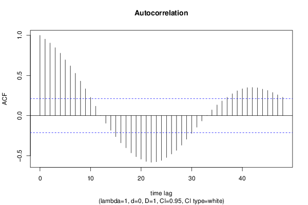
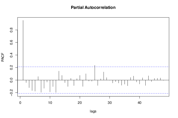
Title produced by software

(Partial) Autocorrelation Function

Date of computation

Tue, 17 Dec 2013 15:27:37 -0500

Cite this page as follows

Statistical Computations at FreeStatistics.org, Office for Research Development and Education, URL https://freestatistics.org/blog/index.php?v=date/2013/Dec/17/t1387312125qh6b9jy23rk9fbk.htm/, Retrieved Fri, 19 Apr 2024 17:54:45 +0000

Statistical Computations at FreeStatistics.org, Office for Research Development and Education, URL https://freestatistics.org/blog/index.php?pk=232420, Retrieved Fri, 19 Apr 2024 17:54:45 +0000

QR Codes:

Paste this QR Code to cite your computation.

Original text written by user:

IsPrivate?

No (this computation is public)

User-defined keywords

Estimated Impact

183

Family? (F = Feedback message, R = changed R code, M = changed R Module, P = changed Parameters, D = changed Data)

-     [Univariate Explorative Data Analysis] [Run Sequence gebo...] [2008-12-12 13:32:37] [76963dc1903f0f612b6153510a3818cf]
- R  D  [Univariate Explorative Data Analysis] [Run Sequence gebo...] [2008-12-17 12:14:40] [76963dc1903f0f612b6153510a3818cf]
-         [Univariate Explorative Data Analysis] [Run Sequence Plot...] [2008-12-22 18:19:51] [1ce0d16c8f4225c977b42c8fa93bc163]
- RMP       [Univariate Data Series] [Identifying Integ...] [2009-11-22 12:08:06] [b98453cac15ba1066b407e146608df68]
- RMP         [(Partial) Autocorrelation Function] [Births] [2010-11-29 09:36:27] [b98453cac15ba1066b407e146608df68]
- R PD          [(Partial) Autocorrelation Function] [ACR 1] [2013-12-03 18:19:48] [0ba55e3ce082ee2313a5fbafd157b436]
-    D              [(Partial) Autocorrelation Function] [autocorrelatie we...] [2013-12-17 20:27:37] [2e4b2f9d3944a9ae720fcdd8099335ae] [Current]

Feedback Forum

Post a new message

Dataseries X:

Download CSV

Histogram

Boxplots

Summary of computational transaction
Raw Input	view raw input (R code)
Raw Output	view raw output of R engine
Computing time	3 seconds
R Server	'Gertrude Mary Cox' @ cox.wessa.net

\begin{tabular}{lllllllll}
\hline
Summary of computational transaction \tabularnewline
Raw Input & view raw input (R code)  \tabularnewline
Raw Output & view raw output of R engine  \tabularnewline
Computing time & 3 seconds \tabularnewline
R Server & 'Gertrude Mary Cox' @ cox.wessa.net \tabularnewline
\hline
\end{tabular}
%Source: https://freestatistics.org/blog/index.php?pk=232420&T=0

[TABLE]
[ROW][C]Summary of computational transaction[/C][/ROW]
[ROW][C]Raw Input[/C][C]view raw input (R code) [/C][/ROW]
[ROW][C]Raw Output[/C][C]view raw output of R engine [/C][/ROW]
[ROW][C]Computing time[/C][C]3 seconds[/C][/ROW]
[ROW][C]R Server[/C][C]'Gertrude Mary Cox' @ cox.wessa.net[/C][/ROW]
[/TABLE]
Source: https://freestatistics.org/blog/index.php?pk=232420&T=0

Globally Unique Identifier (entire table): ba.freestatistics.org/blog/index.php?pk=232420&T=0

As an alternative you can also use a QR Code:

The GUIDs for individual cells are displayed in the table below:

Summary of computational transaction
Raw Input	view raw input (R code)
Raw Output	view raw output of R engine
Computing time	3 seconds
R Server	'Gertrude Mary Cox' @ cox.wessa.net

Autocorrelation Function
Time lag k	ACF(k)	T-STAT	P-value
1	0.952871	8.785	0
2	0.904275	8.337	0
3	0.846915	7.8082	0
4	0.77696	7.1632	0
5	0.694192	6.4001	0
6	0.619097	5.7078	0
7	0.527759	4.8657	3e-06
8	0.429607	3.9608	7.7e-05
9	0.334033	3.0796	0.001396
10	0.227725	2.0995	0.019368
11	0.116722	1.0761	0.142458
12	0.000911	0.0084	0.496658
13	-0.09476	-0.8736	0.192386
14	-0.182351	-1.6812	0.048198
15	-0.262113	-2.4166	0.008904
16	-0.339965	-3.1343	0.001182
17	-0.400874	-3.6959	0.000194
18	-0.464188	-4.2796	2.4e-05
19	-0.512411	-4.7242	5e-06
20	-0.542394	-5.0006	2e-06
21	-0.571121	-5.2655	1e-06
22	-0.581495	-5.3611	0
23	-0.575056	-5.3018	0
24	-0.558348	-5.1477	1e-06
25	-0.521472	-4.8077	3e-06
26	-0.478139	-4.4082	1.5e-05
27	-0.432755	-3.9898	7e-05
28	-0.368474	-3.3972	0.000519
29	-0.294241	-2.7128	0.004038
30	-0.221781	-2.0447	0.021988
31	-0.143951	-1.3272	0.094004
32	-0.066476	-0.6129	0.270797
33	0.003055	0.0282	0.488796
34	0.070823	0.653	0.257772
35	0.133406	1.2299	0.111056
36	0.181571	1.674	0.048903
37	0.227804	2.1002	0.019335
38	0.272157	2.5092	0.007
39	0.309142	2.8501	0.002741
40	0.334528	3.0842	0.001377
41	0.348155	3.2098	0.000937
42	0.350223	3.2289	0.000883
43	0.34669	3.1963	0.000977
44	0.329465	3.0375	0.001584
45	0.313313	2.8886	0.002454
46	0.288172	2.6568	0.00471
47	0.259461	2.3921	0.009478
48	0.228607	2.1077	0.019003

\begin{tabular}{lllllllll}
\hline
Autocorrelation Function \tabularnewline
Time lag k & ACF(k) & T-STAT & P-value \tabularnewline
1 & 0.952871 & 8.785 & 0 \tabularnewline
2 & 0.904275 & 8.337 & 0 \tabularnewline
3 & 0.846915 & 7.8082 & 0 \tabularnewline
4 & 0.77696 & 7.1632 & 0 \tabularnewline
5 & 0.694192 & 6.4001 & 0 \tabularnewline
6 & 0.619097 & 5.7078 & 0 \tabularnewline
7 & 0.527759 & 4.8657 & 3e-06 \tabularnewline
8 & 0.429607 & 3.9608 & 7.7e-05 \tabularnewline
9 & 0.334033 & 3.0796 & 0.001396 \tabularnewline
10 & 0.227725 & 2.0995 & 0.019368 \tabularnewline
11 & 0.116722 & 1.0761 & 0.142458 \tabularnewline
12 & 0.000911 & 0.0084 & 0.496658 \tabularnewline
13 & -0.09476 & -0.8736 & 0.192386 \tabularnewline
14 & -0.182351 & -1.6812 & 0.048198 \tabularnewline
15 & -0.262113 & -2.4166 & 0.008904 \tabularnewline
16 & -0.339965 & -3.1343 & 0.001182 \tabularnewline
17 & -0.400874 & -3.6959 & 0.000194 \tabularnewline
18 & -0.464188 & -4.2796 & 2.4e-05 \tabularnewline
19 & -0.512411 & -4.7242 & 5e-06 \tabularnewline
20 & -0.542394 & -5.0006 & 2e-06 \tabularnewline
21 & -0.571121 & -5.2655 & 1e-06 \tabularnewline
22 & -0.581495 & -5.3611 & 0 \tabularnewline
23 & -0.575056 & -5.3018 & 0 \tabularnewline
24 & -0.558348 & -5.1477 & 1e-06 \tabularnewline
25 & -0.521472 & -4.8077 & 3e-06 \tabularnewline
26 & -0.478139 & -4.4082 & 1.5e-05 \tabularnewline
27 & -0.432755 & -3.9898 & 7e-05 \tabularnewline
28 & -0.368474 & -3.3972 & 0.000519 \tabularnewline
29 & -0.294241 & -2.7128 & 0.004038 \tabularnewline
30 & -0.221781 & -2.0447 & 0.021988 \tabularnewline
31 & -0.143951 & -1.3272 & 0.094004 \tabularnewline
32 & -0.066476 & -0.6129 & 0.270797 \tabularnewline
33 & 0.003055 & 0.0282 & 0.488796 \tabularnewline
34 & 0.070823 & 0.653 & 0.257772 \tabularnewline
35 & 0.133406 & 1.2299 & 0.111056 \tabularnewline
36 & 0.181571 & 1.674 & 0.048903 \tabularnewline
37 & 0.227804 & 2.1002 & 0.019335 \tabularnewline
38 & 0.272157 & 2.5092 & 0.007 \tabularnewline
39 & 0.309142 & 2.8501 & 0.002741 \tabularnewline
40 & 0.334528 & 3.0842 & 0.001377 \tabularnewline
41 & 0.348155 & 3.2098 & 0.000937 \tabularnewline
42 & 0.350223 & 3.2289 & 0.000883 \tabularnewline
43 & 0.34669 & 3.1963 & 0.000977 \tabularnewline
44 & 0.329465 & 3.0375 & 0.001584 \tabularnewline
45 & 0.313313 & 2.8886 & 0.002454 \tabularnewline
46 & 0.288172 & 2.6568 & 0.00471 \tabularnewline
47 & 0.259461 & 2.3921 & 0.009478 \tabularnewline
48 & 0.228607 & 2.1077 & 0.019003 \tabularnewline
\hline
\end{tabular}
%Source: https://freestatistics.org/blog/index.php?pk=232420&T=1

[TABLE]
[ROW][C]Autocorrelation Function[/C][/ROW]
[ROW][C]Time lag k[/C][C]ACF(k)[/C][C]T-STAT[/C][C]P-value[/C][/ROW]
[ROW][C]1[/C][C]0.952871[/C][C]8.785[/C][C]0[/C][/ROW]
[ROW][C]2[/C][C]0.904275[/C][C]8.337[/C][C]0[/C][/ROW]
[ROW][C]3[/C][C]0.846915[/C][C]7.8082[/C][C]0[/C][/ROW]
[ROW][C]4[/C][C]0.77696[/C][C]7.1632[/C][C]0[/C][/ROW]
[ROW][C]5[/C][C]0.694192[/C][C]6.4001[/C][C]0[/C][/ROW]
[ROW][C]6[/C][C]0.619097[/C][C]5.7078[/C][C]0[/C][/ROW]
[ROW][C]7[/C][C]0.527759[/C][C]4.8657[/C][C]3e-06[/C][/ROW]
[ROW][C]8[/C][C]0.429607[/C][C]3.9608[/C][C]7.7e-05[/C][/ROW]
[ROW][C]9[/C][C]0.334033[/C][C]3.0796[/C][C]0.001396[/C][/ROW]
[ROW][C]10[/C][C]0.227725[/C][C]2.0995[/C][C]0.019368[/C][/ROW]
[ROW][C]11[/C][C]0.116722[/C][C]1.0761[/C][C]0.142458[/C][/ROW]
[ROW][C]12[/C][C]0.000911[/C][C]0.0084[/C][C]0.496658[/C][/ROW]
[ROW][C]13[/C][C]-0.09476[/C][C]-0.8736[/C][C]0.192386[/C][/ROW]
[ROW][C]14[/C][C]-0.182351[/C][C]-1.6812[/C][C]0.048198[/C][/ROW]
[ROW][C]15[/C][C]-0.262113[/C][C]-2.4166[/C][C]0.008904[/C][/ROW]
[ROW][C]16[/C][C]-0.339965[/C][C]-3.1343[/C][C]0.001182[/C][/ROW]
[ROW][C]17[/C][C]-0.400874[/C][C]-3.6959[/C][C]0.000194[/C][/ROW]
[ROW][C]18[/C][C]-0.464188[/C][C]-4.2796[/C][C]2.4e-05[/C][/ROW]
[ROW][C]19[/C][C]-0.512411[/C][C]-4.7242[/C][C]5e-06[/C][/ROW]
[ROW][C]20[/C][C]-0.542394[/C][C]-5.0006[/C][C]2e-06[/C][/ROW]
[ROW][C]21[/C][C]-0.571121[/C][C]-5.2655[/C][C]1e-06[/C][/ROW]
[ROW][C]22[/C][C]-0.581495[/C][C]-5.3611[/C][C]0[/C][/ROW]
[ROW][C]23[/C][C]-0.575056[/C][C]-5.3018[/C][C]0[/C][/ROW]
[ROW][C]24[/C][C]-0.558348[/C][C]-5.1477[/C][C]1e-06[/C][/ROW]
[ROW][C]25[/C][C]-0.521472[/C][C]-4.8077[/C][C]3e-06[/C][/ROW]
[ROW][C]26[/C][C]-0.478139[/C][C]-4.4082[/C][C]1.5e-05[/C][/ROW]
[ROW][C]27[/C][C]-0.432755[/C][C]-3.9898[/C][C]7e-05[/C][/ROW]
[ROW][C]28[/C][C]-0.368474[/C][C]-3.3972[/C][C]0.000519[/C][/ROW]
[ROW][C]29[/C][C]-0.294241[/C][C]-2.7128[/C][C]0.004038[/C][/ROW]
[ROW][C]30[/C][C]-0.221781[/C][C]-2.0447[/C][C]0.021988[/C][/ROW]
[ROW][C]31[/C][C]-0.143951[/C][C]-1.3272[/C][C]0.094004[/C][/ROW]
[ROW][C]32[/C][C]-0.066476[/C][C]-0.6129[/C][C]0.270797[/C][/ROW]
[ROW][C]33[/C][C]0.003055[/C][C]0.0282[/C][C]0.488796[/C][/ROW]
[ROW][C]34[/C][C]0.070823[/C][C]0.653[/C][C]0.257772[/C][/ROW]
[ROW][C]35[/C][C]0.133406[/C][C]1.2299[/C][C]0.111056[/C][/ROW]
[ROW][C]36[/C][C]0.181571[/C][C]1.674[/C][C]0.048903[/C][/ROW]
[ROW][C]37[/C][C]0.227804[/C][C]2.1002[/C][C]0.019335[/C][/ROW]
[ROW][C]38[/C][C]0.272157[/C][C]2.5092[/C][C]0.007[/C][/ROW]
[ROW][C]39[/C][C]0.309142[/C][C]2.8501[/C][C]0.002741[/C][/ROW]
[ROW][C]40[/C][C]0.334528[/C][C]3.0842[/C][C]0.001377[/C][/ROW]
[ROW][C]41[/C][C]0.348155[/C][C]3.2098[/C][C]0.000937[/C][/ROW]
[ROW][C]42[/C][C]0.350223[/C][C]3.2289[/C][C]0.000883[/C][/ROW]
[ROW][C]43[/C][C]0.34669[/C][C]3.1963[/C][C]0.000977[/C][/ROW]
[ROW][C]44[/C][C]0.329465[/C][C]3.0375[/C][C]0.001584[/C][/ROW]
[ROW][C]45[/C][C]0.313313[/C][C]2.8886[/C][C]0.002454[/C][/ROW]
[ROW][C]46[/C][C]0.288172[/C][C]2.6568[/C][C]0.00471[/C][/ROW]
[ROW][C]47[/C][C]0.259461[/C][C]2.3921[/C][C]0.009478[/C][/ROW]
[ROW][C]48[/C][C]0.228607[/C][C]2.1077[/C][C]0.019003[/C][/ROW]
[/TABLE]
Source: https://freestatistics.org/blog/index.php?pk=232420&T=1

Globally Unique Identifier (entire table): ba.freestatistics.org/blog/index.php?pk=232420&T=1

As an alternative you can also use a QR Code:

The GUIDs for individual cells are displayed in the table below:

Autocorrelation Function
Time lag k	ACF(k)	T-STAT	P-value
1	0.952871	8.785	0
2	0.904275	8.337	0
3	0.846915	7.8082	0
4	0.77696	7.1632	0
5	0.694192	6.4001	0
6	0.619097	5.7078	0
7	0.527759	4.8657	3e-06
8	0.429607	3.9608	7.7e-05
9	0.334033	3.0796	0.001396
10	0.227725	2.0995	0.019368
11	0.116722	1.0761	0.142458
12	0.000911	0.0084	0.496658
13	-0.09476	-0.8736	0.192386
14	-0.182351	-1.6812	0.048198
15	-0.262113	-2.4166	0.008904
16	-0.339965	-3.1343	0.001182
17	-0.400874	-3.6959	0.000194
18	-0.464188	-4.2796	2.4e-05
19	-0.512411	-4.7242	5e-06
20	-0.542394	-5.0006	2e-06
21	-0.571121	-5.2655	1e-06
22	-0.581495	-5.3611	0
23	-0.575056	-5.3018	0
24	-0.558348	-5.1477	1e-06
25	-0.521472	-4.8077	3e-06
26	-0.478139	-4.4082	1.5e-05
27	-0.432755	-3.9898	7e-05
28	-0.368474	-3.3972	0.000519
29	-0.294241	-2.7128	0.004038
30	-0.221781	-2.0447	0.021988
31	-0.143951	-1.3272	0.094004
32	-0.066476	-0.6129	0.270797
33	0.003055	0.0282	0.488796
34	0.070823	0.653	0.257772
35	0.133406	1.2299	0.111056
36	0.181571	1.674	0.048903
37	0.227804	2.1002	0.019335
38	0.272157	2.5092	0.007
39	0.309142	2.8501	0.002741
40	0.334528	3.0842	0.001377
41	0.348155	3.2098	0.000937
42	0.350223	3.2289	0.000883
43	0.34669	3.1963	0.000977
44	0.329465	3.0375	0.001584
45	0.313313	2.8886	0.002454
46	0.288172	2.6568	0.00471
47	0.259461	2.3921	0.009478
48	0.228607	2.1077	0.019003

Partial Autocorrelation Function
Time lag k	PACF(k)	T-STAT	P-value
1	0.952871	8.785	0
2	-0.040078	-0.3695	0.356337
3	-0.120648	-1.1123	0.134568
4	-0.16796	-1.5485	0.062607
5	-0.177257	-1.6342	0.052955
6	0.05602	0.5165	0.303432
7	-0.194921	-1.7971	0.037937
8	-0.131003	-1.2078	0.115239
9	-0.032209	-0.297	0.383614
10	-0.189171	-1.7441	0.042381
11	-0.104123	-0.96	0.169897
12	-0.196239	-1.8092	0.036975
13	0.143708	1.3249	0.094373
14	0.075502	0.6961	0.244134
15	-0.040849	-0.3766	0.353702
16	-0.102071	-0.941	0.174674
17	0.027948	0.2577	0.398641
18	-0.087681	-0.8084	0.210564
19	0.022771	0.2099	0.41711
20	0.074673	0.6884	0.246523
21	-0.101069	-0.9318	0.177037
22	0.10126	0.9336	0.176584
23	-0.015247	-0.1406	0.444271
24	-0.01849	-0.1705	0.432524
25	0.236285	2.1784	0.016071
26	-0.086391	-0.7965	0.213985
27	0.019576	0.1805	0.428604
28	0.129111	1.1903	0.118613
29	0.039886	0.3677	0.356995
30	-0.002093	-0.0193	0.492326
31	-0.046429	-0.4281	0.334846
32	-0.024536	-0.2262	0.41079
33	-0.047243	-0.4356	0.332131
34	-0.08282	-0.7636	0.22362
35	-0.065384	-0.6028	0.274121
36	-0.090464	-0.834	0.203299
37	0.040741	0.3756	0.35407
38	0.063834	0.5885	0.278872
39	-0.030257	-0.279	0.390478
40	-0.062622	-0.5773	0.282616
41	0.037137	0.3424	0.366454
42	-0.085825	-0.7913	0.215494
43	0.067995	0.6269	0.266209
44	-0.023455	-0.2162	0.414658
45	0.026846	0.2475	0.402556
46	0.029753	0.2743	0.392258
47	0.033981	0.3133	0.377414
48	-0.004415	-0.0407	0.483812

\begin{tabular}{lllllllll}
\hline
Partial Autocorrelation Function \tabularnewline
Time lag k & PACF(k) & T-STAT & P-value \tabularnewline
1 & 0.952871 & 8.785 & 0 \tabularnewline
2 & -0.040078 & -0.3695 & 0.356337 \tabularnewline
3 & -0.120648 & -1.1123 & 0.134568 \tabularnewline
4 & -0.16796 & -1.5485 & 0.062607 \tabularnewline
5 & -0.177257 & -1.6342 & 0.052955 \tabularnewline
6 & 0.05602 & 0.5165 & 0.303432 \tabularnewline
7 & -0.194921 & -1.7971 & 0.037937 \tabularnewline
8 & -0.131003 & -1.2078 & 0.115239 \tabularnewline
9 & -0.032209 & -0.297 & 0.383614 \tabularnewline
10 & -0.189171 & -1.7441 & 0.042381 \tabularnewline
11 & -0.104123 & -0.96 & 0.169897 \tabularnewline
12 & -0.196239 & -1.8092 & 0.036975 \tabularnewline
13 & 0.143708 & 1.3249 & 0.094373 \tabularnewline
14 & 0.075502 & 0.6961 & 0.244134 \tabularnewline
15 & -0.040849 & -0.3766 & 0.353702 \tabularnewline
16 & -0.102071 & -0.941 & 0.174674 \tabularnewline
17 & 0.027948 & 0.2577 & 0.398641 \tabularnewline
18 & -0.087681 & -0.8084 & 0.210564 \tabularnewline
19 & 0.022771 & 0.2099 & 0.41711 \tabularnewline
20 & 0.074673 & 0.6884 & 0.246523 \tabularnewline
21 & -0.101069 & -0.9318 & 0.177037 \tabularnewline
22 & 0.10126 & 0.9336 & 0.176584 \tabularnewline
23 & -0.015247 & -0.1406 & 0.444271 \tabularnewline
24 & -0.01849 & -0.1705 & 0.432524 \tabularnewline
25 & 0.236285 & 2.1784 & 0.016071 \tabularnewline
26 & -0.086391 & -0.7965 & 0.213985 \tabularnewline
27 & 0.019576 & 0.1805 & 0.428604 \tabularnewline
28 & 0.129111 & 1.1903 & 0.118613 \tabularnewline
29 & 0.039886 & 0.3677 & 0.356995 \tabularnewline
30 & -0.002093 & -0.0193 & 0.492326 \tabularnewline
31 & -0.046429 & -0.4281 & 0.334846 \tabularnewline
32 & -0.024536 & -0.2262 & 0.41079 \tabularnewline
33 & -0.047243 & -0.4356 & 0.332131 \tabularnewline
34 & -0.08282 & -0.7636 & 0.22362 \tabularnewline
35 & -0.065384 & -0.6028 & 0.274121 \tabularnewline
36 & -0.090464 & -0.834 & 0.203299 \tabularnewline
37 & 0.040741 & 0.3756 & 0.35407 \tabularnewline
38 & 0.063834 & 0.5885 & 0.278872 \tabularnewline
39 & -0.030257 & -0.279 & 0.390478 \tabularnewline
40 & -0.062622 & -0.5773 & 0.282616 \tabularnewline
41 & 0.037137 & 0.3424 & 0.366454 \tabularnewline
42 & -0.085825 & -0.7913 & 0.215494 \tabularnewline
43 & 0.067995 & 0.6269 & 0.266209 \tabularnewline
44 & -0.023455 & -0.2162 & 0.414658 \tabularnewline
45 & 0.026846 & 0.2475 & 0.402556 \tabularnewline
46 & 0.029753 & 0.2743 & 0.392258 \tabularnewline
47 & 0.033981 & 0.3133 & 0.377414 \tabularnewline
48 & -0.004415 & -0.0407 & 0.483812 \tabularnewline
\hline
\end{tabular}
%Source: https://freestatistics.org/blog/index.php?pk=232420&T=2

[TABLE]
[ROW][C]Partial Autocorrelation Function[/C][/ROW]
[ROW][C]Time lag k[/C][C]PACF(k)[/C][C]T-STAT[/C][C]P-value[/C][/ROW]
[ROW][C]1[/C][C]0.952871[/C][C]8.785[/C][C]0[/C][/ROW]
[ROW][C]2[/C][C]-0.040078[/C][C]-0.3695[/C][C]0.356337[/C][/ROW]
[ROW][C]3[/C][C]-0.120648[/C][C]-1.1123[/C][C]0.134568[/C][/ROW]
[ROW][C]4[/C][C]-0.16796[/C][C]-1.5485[/C][C]0.062607[/C][/ROW]
[ROW][C]5[/C][C]-0.177257[/C][C]-1.6342[/C][C]0.052955[/C][/ROW]
[ROW][C]6[/C][C]0.05602[/C][C]0.5165[/C][C]0.303432[/C][/ROW]
[ROW][C]7[/C][C]-0.194921[/C][C]-1.7971[/C][C]0.037937[/C][/ROW]
[ROW][C]8[/C][C]-0.131003[/C][C]-1.2078[/C][C]0.115239[/C][/ROW]
[ROW][C]9[/C][C]-0.032209[/C][C]-0.297[/C][C]0.383614[/C][/ROW]
[ROW][C]10[/C][C]-0.189171[/C][C]-1.7441[/C][C]0.042381[/C][/ROW]
[ROW][C]11[/C][C]-0.104123[/C][C]-0.96[/C][C]0.169897[/C][/ROW]
[ROW][C]12[/C][C]-0.196239[/C][C]-1.8092[/C][C]0.036975[/C][/ROW]
[ROW][C]13[/C][C]0.143708[/C][C]1.3249[/C][C]0.094373[/C][/ROW]
[ROW][C]14[/C][C]0.075502[/C][C]0.6961[/C][C]0.244134[/C][/ROW]
[ROW][C]15[/C][C]-0.040849[/C][C]-0.3766[/C][C]0.353702[/C][/ROW]
[ROW][C]16[/C][C]-0.102071[/C][C]-0.941[/C][C]0.174674[/C][/ROW]
[ROW][C]17[/C][C]0.027948[/C][C]0.2577[/C][C]0.398641[/C][/ROW]
[ROW][C]18[/C][C]-0.087681[/C][C]-0.8084[/C][C]0.210564[/C][/ROW]
[ROW][C]19[/C][C]0.022771[/C][C]0.2099[/C][C]0.41711[/C][/ROW]
[ROW][C]20[/C][C]0.074673[/C][C]0.6884[/C][C]0.246523[/C][/ROW]
[ROW][C]21[/C][C]-0.101069[/C][C]-0.9318[/C][C]0.177037[/C][/ROW]
[ROW][C]22[/C][C]0.10126[/C][C]0.9336[/C][C]0.176584[/C][/ROW]
[ROW][C]23[/C][C]-0.015247[/C][C]-0.1406[/C][C]0.444271[/C][/ROW]
[ROW][C]24[/C][C]-0.01849[/C][C]-0.1705[/C][C]0.432524[/C][/ROW]
[ROW][C]25[/C][C]0.236285[/C][C]2.1784[/C][C]0.016071[/C][/ROW]
[ROW][C]26[/C][C]-0.086391[/C][C]-0.7965[/C][C]0.213985[/C][/ROW]
[ROW][C]27[/C][C]0.019576[/C][C]0.1805[/C][C]0.428604[/C][/ROW]
[ROW][C]28[/C][C]0.129111[/C][C]1.1903[/C][C]0.118613[/C][/ROW]
[ROW][C]29[/C][C]0.039886[/C][C]0.3677[/C][C]0.356995[/C][/ROW]
[ROW][C]30[/C][C]-0.002093[/C][C]-0.0193[/C][C]0.492326[/C][/ROW]
[ROW][C]31[/C][C]-0.046429[/C][C]-0.4281[/C][C]0.334846[/C][/ROW]
[ROW][C]32[/C][C]-0.024536[/C][C]-0.2262[/C][C]0.41079[/C][/ROW]
[ROW][C]33[/C][C]-0.047243[/C][C]-0.4356[/C][C]0.332131[/C][/ROW]
[ROW][C]34[/C][C]-0.08282[/C][C]-0.7636[/C][C]0.22362[/C][/ROW]
[ROW][C]35[/C][C]-0.065384[/C][C]-0.6028[/C][C]0.274121[/C][/ROW]
[ROW][C]36[/C][C]-0.090464[/C][C]-0.834[/C][C]0.203299[/C][/ROW]
[ROW][C]37[/C][C]0.040741[/C][C]0.3756[/C][C]0.35407[/C][/ROW]
[ROW][C]38[/C][C]0.063834[/C][C]0.5885[/C][C]0.278872[/C][/ROW]
[ROW][C]39[/C][C]-0.030257[/C][C]-0.279[/C][C]0.390478[/C][/ROW]
[ROW][C]40[/C][C]-0.062622[/C][C]-0.5773[/C][C]0.282616[/C][/ROW]
[ROW][C]41[/C][C]0.037137[/C][C]0.3424[/C][C]0.366454[/C][/ROW]
[ROW][C]42[/C][C]-0.085825[/C][C]-0.7913[/C][C]0.215494[/C][/ROW]
[ROW][C]43[/C][C]0.067995[/C][C]0.6269[/C][C]0.266209[/C][/ROW]
[ROW][C]44[/C][C]-0.023455[/C][C]-0.2162[/C][C]0.414658[/C][/ROW]
[ROW][C]45[/C][C]0.026846[/C][C]0.2475[/C][C]0.402556[/C][/ROW]
[ROW][C]46[/C][C]0.029753[/C][C]0.2743[/C][C]0.392258[/C][/ROW]
[ROW][C]47[/C][C]0.033981[/C][C]0.3133[/C][C]0.377414[/C][/ROW]
[ROW][C]48[/C][C]-0.004415[/C][C]-0.0407[/C][C]0.483812[/C][/ROW]
[/TABLE]
Source: https://freestatistics.org/blog/index.php?pk=232420&T=2

Globally Unique Identifier (entire table): ba.freestatistics.org/blog/index.php?pk=232420&T=2

As an alternative you can also use a QR Code:

The GUIDs for individual cells are displayed in the table below:

Partial Autocorrelation Function
Time lag k	PACF(k)	T-STAT	P-value
1	0.952871	8.785	0
2	-0.040078	-0.3695	0.356337
3	-0.120648	-1.1123	0.134568
4	-0.16796	-1.5485	0.062607
5	-0.177257	-1.6342	0.052955
6	0.05602	0.5165	0.303432
7	-0.194921	-1.7971	0.037937
8	-0.131003	-1.2078	0.115239
9	-0.032209	-0.297	0.383614
10	-0.189171	-1.7441	0.042381
11	-0.104123	-0.96	0.169897
12	-0.196239	-1.8092	0.036975
13	0.143708	1.3249	0.094373
14	0.075502	0.6961	0.244134
15	-0.040849	-0.3766	0.353702
16	-0.102071	-0.941	0.174674
17	0.027948	0.2577	0.398641
18	-0.087681	-0.8084	0.210564
19	0.022771	0.2099	0.41711
20	0.074673	0.6884	0.246523
21	-0.101069	-0.9318	0.177037
22	0.10126	0.9336	0.176584
23	-0.015247	-0.1406	0.444271
24	-0.01849	-0.1705	0.432524
25	0.236285	2.1784	0.016071
26	-0.086391	-0.7965	0.213985
27	0.019576	0.1805	0.428604
28	0.129111	1.1903	0.118613
29	0.039886	0.3677	0.356995
30	-0.002093	-0.0193	0.492326
31	-0.046429	-0.4281	0.334846
32	-0.024536	-0.2262	0.41079
33	-0.047243	-0.4356	0.332131
34	-0.08282	-0.7636	0.22362
35	-0.065384	-0.6028	0.274121
36	-0.090464	-0.834	0.203299
37	0.040741	0.3756	0.35407
38	0.063834	0.5885	0.278872
39	-0.030257	-0.279	0.390478
40	-0.062622	-0.5773	0.282616
41	0.037137	0.3424	0.366454
42	-0.085825	-0.7913	0.215494
43	0.067995	0.6269	0.266209
44	-0.023455	-0.2162	0.414658
45	0.026846	0.2475	0.402556
46	0.029753	0.2743	0.392258
47	0.033981	0.3133	0.377414
48	-0.004415	-0.0407	0.483812

Figure 1

PNG link

Postscript link

PDF link

Figure 2

PNG link

Postscript link

PDF link

Parameters (Session):

par1 = 48 ; par2 = 1 ; par3 = 0 ; par4 = 1 ; par5 = 12 ; par6 = White Noise ; par7 = 0.95 ;

Parameters (R input):

par1 = 48 ; par2 = 1 ; par3 = 0 ; par4 = 1 ; par5 = 12 ; par6 = White Noise ; par7 = 0.95 ; par8 = ;

R code (references can be found in the software module):

if (par1 == 'Default') {
par1 = 10*log10(length(x))
} else {
par1 <- as.numeric(par1)
}
par2 <- as.numeric(par2)
par3 <- as.numeric(par3)
par4 <- as.numeric(par4)
par5 <- as.numeric(par5)
if (par6 == 'White Noise') par6 <- 'white' else par6 <- 'ma'
par7 <- as.numeric(par7)
if (par2 == 0) {
x <- log(x)
} else {
x <- (x ^ par2 - 1) / par2
}
if (par3 > 0) x <- diff(x,lag=1,difference=par3)
if (par4 > 0) x <- diff(x,lag=par5,difference=par4)
bitmap(file='pic1.png')
racf <- acf(x, par1, main='Autocorrelation', xlab='time lag', ylab='ACF', ci.type=par6, ci=par7, sub=paste('(lambda=',par2,', d=',par3,', D=',par4,', CI=', par7, ', CI type=',par6,')',sep=''))
dev.off()
bitmap(file='pic2.png')
rpacf <- pacf(x,par1,main='Partial Autocorrelation',xlab='lags',ylab='PACF')
dev.off()
(myacf <- c(racf$acf))
(mypacf <- c(rpacf$acf))
lengthx <- length(x)
sqrtn <- sqrt(lengthx)
load(file='createtable')
a<-table.start()
a<-table.row.start(a)
a<-table.element(a,'Autocorrelation Function',4,TRUE)
a<-table.row.end(a)
a<-table.row.start(a)
a<-table.element(a,'Time lag k',header=TRUE)
a<-table.element(a,hyperlink('basics.htm','ACF(k)','click here for more information about the Autocorrelation Function'),header=TRUE)
a<-table.element(a,'T-STAT',header=TRUE)
a<-table.element(a,'P-value',header=TRUE)
a<-table.row.end(a)
for (i in 2:(par1+1)) {
a<-table.row.start(a)
a<-table.element(a,i-1,header=TRUE)
a<-table.element(a,round(myacf[i],6))
mytstat <- myacf[i]*sqrtn
a<-table.element(a,round(mytstat,4))
a<-table.element(a,round(1-pt(abs(mytstat),lengthx),6))
a<-table.row.end(a)
}
a<-table.end(a)
table.save(a,file='mytable.tab')
a<-table.start()
a<-table.row.start(a)
a<-table.element(a,'Partial Autocorrelation Function',4,TRUE)
a<-table.row.end(a)
a<-table.row.start(a)
a<-table.element(a,'Time lag k',header=TRUE)
a<-table.element(a,hyperlink('basics.htm','PACF(k)','click here for more information about the Partial Autocorrelation Function'),header=TRUE)
a<-table.element(a,'T-STAT',header=TRUE)
a<-table.element(a,'P-value',header=TRUE)
a<-table.row.end(a)
for (i in 1:par1) {
a<-table.row.start(a)
a<-table.element(a,i,header=TRUE)
a<-table.element(a,round(mypacf[i],6))
mytstat <- mypacf[i]*sqrtn
a<-table.element(a,round(mytstat,4))
a<-table.element(a,round(1-pt(abs(mytstat),lengthx),6))
a<-table.row.end(a)
}
a<-table.end(a)
table.save(a,file='mytable1.tab')

Free Statistics

Description of Statistical Computation

Tree of Dependent Computations

Dataset

Tables (Output of Computation)

Figures (Output of Computation)

Input Parameters & R Code