Free Statistics
of Irreproducible Research!
Description of Statistical Computation | |||||||||||||||||||||||||||||||||||||||||||||||||||||||||||||||||||||||||||||||||||||||||||||||||||||||||||||||||||||||||||||||||||||||||||||||||||||||||||||||||||||||||||||||||||||||||||||||||||||||||||||||||||||||||||||||||||||||||||||||||||||||||||||||||||||||||||||||||||||||||||||||||||||||||||||||||||||||||||||||||||||||||||||||||||||||||||||||||||||||||||||||||||||||||||||||||||||||||||||||||||||||||||||||||||||||||||||||||||||||||||||||||||||||||||||||||||||||||||||||||||||||||||||
|---|---|---|---|---|---|---|---|---|---|---|---|---|---|---|---|---|---|---|---|---|---|---|---|---|---|---|---|---|---|---|---|---|---|---|---|---|---|---|---|---|---|---|---|---|---|---|---|---|---|---|---|---|---|---|---|---|---|---|---|---|---|---|---|---|---|---|---|---|---|---|---|---|---|---|---|---|---|---|---|---|---|---|---|---|---|---|---|---|---|---|---|---|---|---|---|---|---|---|---|---|---|---|---|---|---|---|---|---|---|---|---|---|---|---|---|---|---|---|---|---|---|---|---|---|---|---|---|---|---|---|---|---|---|---|---|---|---|---|---|---|---|---|---|---|---|---|---|---|---|---|---|---|---|---|---|---|---|---|---|---|---|---|---|---|---|---|---|---|---|---|---|---|---|---|---|---|---|---|---|---|---|---|---|---|---|---|---|---|---|---|---|---|---|---|---|---|---|---|---|---|---|---|---|---|---|---|---|---|---|---|---|---|---|---|---|---|---|---|---|---|---|---|---|---|---|---|---|---|---|---|---|---|---|---|---|---|---|---|---|---|---|---|---|---|---|---|---|---|---|---|---|---|---|---|---|---|---|---|---|---|---|---|---|---|---|---|---|---|---|---|---|---|---|---|---|---|---|---|---|---|---|---|---|---|---|---|---|---|---|---|---|---|---|---|---|---|---|---|---|---|---|---|---|---|---|---|---|---|---|---|---|---|---|---|---|---|---|---|---|---|---|---|---|---|---|---|---|---|---|---|---|---|---|---|---|---|---|---|---|---|---|---|---|---|---|---|---|---|---|---|---|---|---|---|---|---|---|---|---|---|---|---|---|---|---|---|---|---|---|---|---|---|---|---|---|---|---|---|---|---|---|---|---|---|---|---|---|---|---|---|---|---|---|---|---|---|---|---|---|---|---|---|---|---|---|---|---|---|---|---|---|---|---|---|---|---|---|---|---|---|---|---|---|---|---|---|---|---|---|---|---|---|---|---|---|---|---|---|---|---|---|---|---|---|---|---|---|---|---|---|---|---|---|---|---|---|---|---|---|---|---|---|---|---|---|---|---|---|---|---|---|---|---|---|---|---|---|---|---|---|---|---|---|---|---|---|---|---|---|---|---|---|---|
| Author's title | |||||||||||||||||||||||||||||||||||||||||||||||||||||||||||||||||||||||||||||||||||||||||||||||||||||||||||||||||||||||||||||||||||||||||||||||||||||||||||||||||||||||||||||||||||||||||||||||||||||||||||||||||||||||||||||||||||||||||||||||||||||||||||||||||||||||||||||||||||||||||||||||||||||||||||||||||||||||||||||||||||||||||||||||||||||||||||||||||||||||||||||||||||||||||||||||||||||||||||||||||||||||||||||||||||||||||||||||||||||||||||||||||||||||||||||||||||||||||||||||||||||||||||||
| Author | *The author of this computation has been verified* | ||||||||||||||||||||||||||||||||||||||||||||||||||||||||||||||||||||||||||||||||||||||||||||||||||||||||||||||||||||||||||||||||||||||||||||||||||||||||||||||||||||||||||||||||||||||||||||||||||||||||||||||||||||||||||||||||||||||||||||||||||||||||||||||||||||||||||||||||||||||||||||||||||||||||||||||||||||||||||||||||||||||||||||||||||||||||||||||||||||||||||||||||||||||||||||||||||||||||||||||||||||||||||||||||||||||||||||||||||||||||||||||||||||||||||||||||||||||||||||||||||||||||||||
| R Software Module | rwasp_pairs.wasp | ||||||||||||||||||||||||||||||||||||||||||||||||||||||||||||||||||||||||||||||||||||||||||||||||||||||||||||||||||||||||||||||||||||||||||||||||||||||||||||||||||||||||||||||||||||||||||||||||||||||||||||||||||||||||||||||||||||||||||||||||||||||||||||||||||||||||||||||||||||||||||||||||||||||||||||||||||||||||||||||||||||||||||||||||||||||||||||||||||||||||||||||||||||||||||||||||||||||||||||||||||||||||||||||||||||||||||||||||||||||||||||||||||||||||||||||||||||||||||||||||||||||||||||
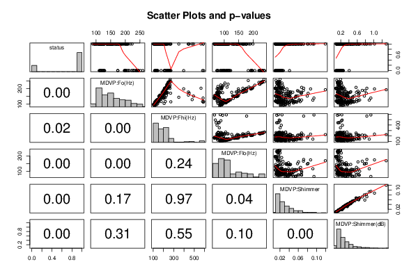
| Title produced by software | Kendall tau Correlation Matrix | ||||||||||||||||||||||||||||||||||||||||||||||||||||||||||||||||||||||||||||||||||||||||||||||||||||||||||||||||||||||||||||||||||||||||||||||||||||||||||||||||||||||||||||||||||||||||||||||||||||||||||||||||||||||||||||||||||||||||||||||||||||||||||||||||||||||||||||||||||||||||||||||||||||||||||||||||||||||||||||||||||||||||||||||||||||||||||||||||||||||||||||||||||||||||||||||||||||||||||||||||||||||||||||||||||||||||||||||||||||||||||||||||||||||||||||||||||||||||||||||||||||||||||||
| Date of computation | Sun, 08 Dec 2013 11:25:57 -0500 | ||||||||||||||||||||||||||||||||||||||||||||||||||||||||||||||||||||||||||||||||||||||||||||||||||||||||||||||||||||||||||||||||||||||||||||||||||||||||||||||||||||||||||||||||||||||||||||||||||||||||||||||||||||||||||||||||||||||||||||||||||||||||||||||||||||||||||||||||||||||||||||||||||||||||||||||||||||||||||||||||||||||||||||||||||||||||||||||||||||||||||||||||||||||||||||||||||||||||||||||||||||||||||||||||||||||||||||||||||||||||||||||||||||||||||||||||||||||||||||||||||||||||||||
| Cite this page as follows | Statistical Computations at FreeStatistics.org, Office for Research Development and Education, URL https://freestatistics.org/blog/index.php?v=date/2013/Dec/08/t1386519970rqmwq0cv5fpop8h.htm/, Retrieved Fri, 19 Apr 2024 01:01:53 +0000 | ||||||||||||||||||||||||||||||||||||||||||||||||||||||||||||||||||||||||||||||||||||||||||||||||||||||||||||||||||||||||||||||||||||||||||||||||||||||||||||||||||||||||||||||||||||||||||||||||||||||||||||||||||||||||||||||||||||||||||||||||||||||||||||||||||||||||||||||||||||||||||||||||||||||||||||||||||||||||||||||||||||||||||||||||||||||||||||||||||||||||||||||||||||||||||||||||||||||||||||||||||||||||||||||||||||||||||||||||||||||||||||||||||||||||||||||||||||||||||||||||||||||||||||
| Statistical Computations at FreeStatistics.org, Office for Research Development and Education, URL https://freestatistics.org/blog/index.php?pk=231471, Retrieved Fri, 19 Apr 2024 01:01:53 +0000 | |||||||||||||||||||||||||||||||||||||||||||||||||||||||||||||||||||||||||||||||||||||||||||||||||||||||||||||||||||||||||||||||||||||||||||||||||||||||||||||||||||||||||||||||||||||||||||||||||||||||||||||||||||||||||||||||||||||||||||||||||||||||||||||||||||||||||||||||||||||||||||||||||||||||||||||||||||||||||||||||||||||||||||||||||||||||||||||||||||||||||||||||||||||||||||||||||||||||||||||||||||||||||||||||||||||||||||||||||||||||||||||||||||||||||||||||||||||||||||||||||||||||||||||
| QR Codes: | |||||||||||||||||||||||||||||||||||||||||||||||||||||||||||||||||||||||||||||||||||||||||||||||||||||||||||||||||||||||||||||||||||||||||||||||||||||||||||||||||||||||||||||||||||||||||||||||||||||||||||||||||||||||||||||||||||||||||||||||||||||||||||||||||||||||||||||||||||||||||||||||||||||||||||||||||||||||||||||||||||||||||||||||||||||||||||||||||||||||||||||||||||||||||||||||||||||||||||||||||||||||||||||||||||||||||||||||||||||||||||||||||||||||||||||||||||||||||||||||||||||||||||||
|
| |||||||||||||||||||||||||||||||||||||||||||||||||||||||||||||||||||||||||||||||||||||||||||||||||||||||||||||||||||||||||||||||||||||||||||||||||||||||||||||||||||||||||||||||||||||||||||||||||||||||||||||||||||||||||||||||||||||||||||||||||||||||||||||||||||||||||||||||||||||||||||||||||||||||||||||||||||||||||||||||||||||||||||||||||||||||||||||||||||||||||||||||||||||||||||||||||||||||||||||||||||||||||||||||||||||||||||||||||||||||||||||||||||||||||||||||||||||||||||||||||||||||||||||
| Original text written by user: | |||||||||||||||||||||||||||||||||||||||||||||||||||||||||||||||||||||||||||||||||||||||||||||||||||||||||||||||||||||||||||||||||||||||||||||||||||||||||||||||||||||||||||||||||||||||||||||||||||||||||||||||||||||||||||||||||||||||||||||||||||||||||||||||||||||||||||||||||||||||||||||||||||||||||||||||||||||||||||||||||||||||||||||||||||||||||||||||||||||||||||||||||||||||||||||||||||||||||||||||||||||||||||||||||||||||||||||||||||||||||||||||||||||||||||||||||||||||||||||||||||||||||||||
| IsPrivate? | No (this computation is public) | ||||||||||||||||||||||||||||||||||||||||||||||||||||||||||||||||||||||||||||||||||||||||||||||||||||||||||||||||||||||||||||||||||||||||||||||||||||||||||||||||||||||||||||||||||||||||||||||||||||||||||||||||||||||||||||||||||||||||||||||||||||||||||||||||||||||||||||||||||||||||||||||||||||||||||||||||||||||||||||||||||||||||||||||||||||||||||||||||||||||||||||||||||||||||||||||||||||||||||||||||||||||||||||||||||||||||||||||||||||||||||||||||||||||||||||||||||||||||||||||||||||||||||||
| User-defined keywords | |||||||||||||||||||||||||||||||||||||||||||||||||||||||||||||||||||||||||||||||||||||||||||||||||||||||||||||||||||||||||||||||||||||||||||||||||||||||||||||||||||||||||||||||||||||||||||||||||||||||||||||||||||||||||||||||||||||||||||||||||||||||||||||||||||||||||||||||||||||||||||||||||||||||||||||||||||||||||||||||||||||||||||||||||||||||||||||||||||||||||||||||||||||||||||||||||||||||||||||||||||||||||||||||||||||||||||||||||||||||||||||||||||||||||||||||||||||||||||||||||||||||||||||
| Estimated Impact | 105 | ||||||||||||||||||||||||||||||||||||||||||||||||||||||||||||||||||||||||||||||||||||||||||||||||||||||||||||||||||||||||||||||||||||||||||||||||||||||||||||||||||||||||||||||||||||||||||||||||||||||||||||||||||||||||||||||||||||||||||||||||||||||||||||||||||||||||||||||||||||||||||||||||||||||||||||||||||||||||||||||||||||||||||||||||||||||||||||||||||||||||||||||||||||||||||||||||||||||||||||||||||||||||||||||||||||||||||||||||||||||||||||||||||||||||||||||||||||||||||||||||||||||||||||
Tree of Dependent Computations | |||||||||||||||||||||||||||||||||||||||||||||||||||||||||||||||||||||||||||||||||||||||||||||||||||||||||||||||||||||||||||||||||||||||||||||||||||||||||||||||||||||||||||||||||||||||||||||||||||||||||||||||||||||||||||||||||||||||||||||||||||||||||||||||||||||||||||||||||||||||||||||||||||||||||||||||||||||||||||||||||||||||||||||||||||||||||||||||||||||||||||||||||||||||||||||||||||||||||||||||||||||||||||||||||||||||||||||||||||||||||||||||||||||||||||||||||||||||||||||||||||||||||||||
| Family? (F = Feedback message, R = changed R code, M = changed R Module, P = changed Parameters, D = changed Data) | |||||||||||||||||||||||||||||||||||||||||||||||||||||||||||||||||||||||||||||||||||||||||||||||||||||||||||||||||||||||||||||||||||||||||||||||||||||||||||||||||||||||||||||||||||||||||||||||||||||||||||||||||||||||||||||||||||||||||||||||||||||||||||||||||||||||||||||||||||||||||||||||||||||||||||||||||||||||||||||||||||||||||||||||||||||||||||||||||||||||||||||||||||||||||||||||||||||||||||||||||||||||||||||||||||||||||||||||||||||||||||||||||||||||||||||||||||||||||||||||||||||||||||||
| - [Kendall tau Correlation Matrix] [] [2010-12-05 17:44:33] [b98453cac15ba1066b407e146608df68] - RMPD [Kendall tau Correlation Matrix] [] [2013-12-08 16:25:57] [05fc9f73518f9509c56332c989d681e3] [Current] | |||||||||||||||||||||||||||||||||||||||||||||||||||||||||||||||||||||||||||||||||||||||||||||||||||||||||||||||||||||||||||||||||||||||||||||||||||||||||||||||||||||||||||||||||||||||||||||||||||||||||||||||||||||||||||||||||||||||||||||||||||||||||||||||||||||||||||||||||||||||||||||||||||||||||||||||||||||||||||||||||||||||||||||||||||||||||||||||||||||||||||||||||||||||||||||||||||||||||||||||||||||||||||||||||||||||||||||||||||||||||||||||||||||||||||||||||||||||||||||||||||||||||||||
| Feedback Forum | |||||||||||||||||||||||||||||||||||||||||||||||||||||||||||||||||||||||||||||||||||||||||||||||||||||||||||||||||||||||||||||||||||||||||||||||||||||||||||||||||||||||||||||||||||||||||||||||||||||||||||||||||||||||||||||||||||||||||||||||||||||||||||||||||||||||||||||||||||||||||||||||||||||||||||||||||||||||||||||||||||||||||||||||||||||||||||||||||||||||||||||||||||||||||||||||||||||||||||||||||||||||||||||||||||||||||||||||||||||||||||||||||||||||||||||||||||||||||||||||||||||||||||||
Post a new message | |||||||||||||||||||||||||||||||||||||||||||||||||||||||||||||||||||||||||||||||||||||||||||||||||||||||||||||||||||||||||||||||||||||||||||||||||||||||||||||||||||||||||||||||||||||||||||||||||||||||||||||||||||||||||||||||||||||||||||||||||||||||||||||||||||||||||||||||||||||||||||||||||||||||||||||||||||||||||||||||||||||||||||||||||||||||||||||||||||||||||||||||||||||||||||||||||||||||||||||||||||||||||||||||||||||||||||||||||||||||||||||||||||||||||||||||||||||||||||||||||||||||||||||
Dataset | |||||||||||||||||||||||||||||||||||||||||||||||||||||||||||||||||||||||||||||||||||||||||||||||||||||||||||||||||||||||||||||||||||||||||||||||||||||||||||||||||||||||||||||||||||||||||||||||||||||||||||||||||||||||||||||||||||||||||||||||||||||||||||||||||||||||||||||||||||||||||||||||||||||||||||||||||||||||||||||||||||||||||||||||||||||||||||||||||||||||||||||||||||||||||||||||||||||||||||||||||||||||||||||||||||||||||||||||||||||||||||||||||||||||||||||||||||||||||||||||||||||||||||||
| Dataseries X: | |||||||||||||||||||||||||||||||||||||||||||||||||||||||||||||||||||||||||||||||||||||||||||||||||||||||||||||||||||||||||||||||||||||||||||||||||||||||||||||||||||||||||||||||||||||||||||||||||||||||||||||||||||||||||||||||||||||||||||||||||||||||||||||||||||||||||||||||||||||||||||||||||||||||||||||||||||||||||||||||||||||||||||||||||||||||||||||||||||||||||||||||||||||||||||||||||||||||||||||||||||||||||||||||||||||||||||||||||||||||||||||||||||||||||||||||||||||||||||||||||||||||||||||
1 119.992 157.302 74.997 0.04374 0.426 1 122.4 148.65 113.819 0.06134 0.626 1 116.682 131.111 111.555 0.05233 0.482 1 116.676 137.871 111.366 0.05492 0.517 1 116.014 141.781 110.655 0.06425 0.584 1 120.552 131.162 113.787 0.04701 0.456 1 120.267 137.244 114.82 0.01608 0.14 1 107.332 113.84 104.315 0.01567 0.134 1 95.73 132.068 91.754 0.02093 0.191 1 95.056 120.103 91.226 0.02838 0.255 1 88.333 112.24 84.072 0.02143 0.197 1 91.904 115.871 86.292 0.02752 0.249 1 136.926 159.866 131.276 0.01259 0.112 1 139.173 179.139 76.556 0.01642 0.154 1 152.845 163.305 75.836 0.01828 0.158 1 142.167 217.455 83.159 0.01503 0.126 1 144.188 349.259 82.764 0.02047 0.192 1 168.778 232.181 75.603 0.03327 0.348 1 153.046 175.829 68.623 0.05517 0.542 1 156.405 189.398 142.822 0.03995 0.348 1 153.848 165.738 65.782 0.0381 0.328 1 153.88 172.86 78.128 0.04137 0.37 1 167.93 193.221 79.068 0.04351 0.377 1 173.917 192.735 86.18 0.04192 0.364 1 163.656 200.841 76.779 0.01659 0.164 1 104.4 206.002 77.968 0.03767 0.381 1 171.041 208.313 75.501 0.01966 0.186 1 146.845 208.701 81.737 0.01919 0.198 1 155.358 227.383 80.055 0.01718 0.161 1 162.568 198.346 77.63 0.01791 0.168 0 197.076 206.896 192.055 0.01098 0.097 0 199.228 209.512 192.091 0.01015 0.089 0 198.383 215.203 193.104 0.01263 0.111 0 202.266 211.604 197.079 0.00954 0.085 0 203.184 211.526 196.16 0.00958 0.085 0 201.464 210.565 195.708 0.01194 0.107 1 177.876 192.921 168.013 0.02126 0.189 1 176.17 185.604 163.564 0.01851 0.168 1 180.198 201.249 175.456 0.01444 0.131 1 187.733 202.324 173.015 0.01663 0.151 1 186.163 197.724 177.584 0.01495 0.135 1 184.055 196.537 166.977 0.01463 0.132 0 237.226 247.326 225.227 0.01752 0.164 0 241.404 248.834 232.483 0.0176 0.154 0 243.439 250.912 232.435 0.01419 0.126 0 242.852 255.034 227.911 0.01494 0.134 0 245.51 262.09 231.848 0.01608 0.141 0 252.455 261.487 182.786 0.01152 0.103 0 122.188 128.611 115.765 0.01613 0.143 0 122.964 130.049 114.676 0.01681 0.154 0 124.445 135.069 117.495 0.02184 0.197 0 126.344 134.231 112.773 0.02033 0.185 0 128.001 138.052 122.08 0.02297 0.21 0 129.336 139.867 118.604 0.02498 0.228 1 108.807 134.656 102.874 0.02719 0.255 1 109.86 126.358 104.437 0.03209 0.307 1 110.417 131.067 103.37 0.03715 0.334 1 117.274 129.916 110.402 0.02293 0.221 1 116.879 131.897 108.153 0.02645 0.265 1 114.847 271.314 104.68 0.03225 0.35 0 209.144 237.494 109.379 0.01861 0.17 0 223.365 238.987 98.664 0.01906 0.165 0 222.236 231.345 205.495 0.01643 0.145 0 228.832 234.619 223.634 0.01644 0.145 0 229.401 252.221 221.156 0.01457 0.129 0 228.969 239.541 113.201 0.01745 0.154 1 140.341 159.774 67.021 0.03198 0.313 1 136.969 166.607 66.004 0.03111 0.308 1 143.533 162.215 65.809 0.05384 0.478 1 148.09 162.824 67.343 0.05428 0.497 1 142.729 162.408 65.476 0.03485 0.365 1 136.358 176.595 65.75 0.04978 0.483 1 120.08 139.71 111.208 0.01706 0.152 1 112.014 588.518 107.024 0.02448 0.226 1 110.793 128.101 107.316 0.02442 0.216 1 110.707 122.611 105.007 0.02215 0.206 1 112.876 148.826 106.981 0.03999 0.35 1 110.568 125.394 106.821 0.02199 0.197 1 95.385 102.145 90.264 0.03202 0.263 1 100.77 115.697 85.545 0.03121 0.361 1 96.106 108.664 84.51 0.04024 0.364 1 95.605 107.715 87.549 0.03156 0.296 1 100.96 110.019 95.628 0.02427 0.216 1 98.804 102.305 87.804 0.02223 0.202 1 176.858 205.56 75.344 0.04795 0.435 1 180.978 200.125 155.495 0.03852 0.331 1 178.222 202.45 141.047 0.03759 0.327 1 176.281 227.381 125.61 0.06511 0.58 1 173.898 211.35 74.677 0.06727 0.65 1 179.711 225.93 144.878 0.04313 0.442 1 166.605 206.008 78.032 0.0664 0.634 1 151.955 163.335 147.226 0.07959 0.772 1 148.272 164.989 142.299 0.0419 0.383 1 152.125 161.469 76.596 0.05925 0.637 1 157.821 172.975 68.401 0.03716 0.307 1 157.447 163.267 149.605 0.03272 0.283 1 159.116 168.913 144.811 0.03381 0.307 1 125.036 143.946 116.187 0.03886 0.342 1 125.791 140.557 96.206 0.04689 0.422 1 126.512 141.756 99.77 0.06734 0.659 1 125.641 141.068 116.346 0.09178 0.891 1 128.451 150.449 75.632 0.0617 0.584 1 139.224 586.567 66.157 0.09419 0.93 1 150.258 154.609 75.349 0.01131 0.107 1 154.003 160.267 128.621 0.0103 0.094 1 149.689 160.368 133.608 0.01346 0.126 1 155.078 163.736 144.148 0.01064 0.097 1 151.884 157.765 133.751 0.0145 0.137 1 151.989 157.339 132.857 0.01024 0.093 1 193.03 208.9 80.297 0.03044 0.275 1 200.714 223.982 89.686 0.02286 0.207 1 208.519 220.315 199.02 0.01761 0.155 1 204.664 221.3 189.621 0.02378 0.21 1 210.141 232.706 185.258 0.0168 0.149 1 206.327 226.355 92.02 0.02105 0.209 1 151.872 492.892 69.085 0.01843 0.235 1 158.219 442.557 71.948 0.01458 0.148 1 170.756 450.247 79.032 0.01725 0.175 1 178.285 442.824 82.063 0.01279 0.129 1 217.116 233.481 93.978 0.01299 0.124 1 128.94 479.697 88.251 0.02008 0.221 1 176.824 215.293 83.961 0.01169 0.117 1 138.19 203.522 83.34 0.04479 0.441 1 182.018 197.173 79.187 0.02503 0.231 1 156.239 195.107 79.82 0.02343 0.224 1 145.174 198.109 80.637 0.02362 0.233 1 138.145 197.238 81.114 0.02791 0.246 1 166.888 198.966 79.512 0.02857 0.257 1 119.031 127.533 109.216 0.01033 0.098 1 120.078 126.632 105.667 0.01022 0.09 1 120.289 128.143 100.209 0.01412 0.125 1 120.256 125.306 104.773 0.01516 0.138 1 119.056 125.213 86.795 0.01201 0.106 1 118.747 123.723 109.836 0.01043 0.099 1 106.516 112.777 93.105 0.04932 0.441 1 110.453 127.611 105.554 0.04128 0.379 1 113.4 133.344 107.816 0.04879 0.431 1 113.166 130.27 100.673 0.05279 0.476 1 112.239 126.609 104.095 0.05643 0.517 1 116.15 131.731 109.815 0.03026 0.267 1 170.368 268.796 79.543 0.03273 0.281 1 208.083 253.792 91.802 0.06725 0.571 1 198.458 219.29 148.691 0.03527 0.297 1 202.805 231.508 86.232 0.01997 0.18 1 202.544 241.35 164.168 0.02662 0.228 1 223.361 263.872 87.638 0.02536 0.225 1 169.774 191.759 151.451 0.08143 0.821 1 183.52 216.814 161.34 0.0605 0.618 1 188.62 216.302 165.982 0.07118 0.722 1 202.632 565.74 177.258 0.0717 0.833 1 186.695 211.961 149.442 0.0583 0.784 1 192.818 224.429 168.793 0.11908 1.302 1 198.116 233.099 174.478 0.08684 1.018 1 121.345 139.644 98.25 0.02534 0.241 1 119.1 128.442 88.833 0.02682 0.236 1 117.87 127.349 95.654 0.03087 0.276 1 122.336 142.369 94.794 0.02293 0.223 1 117.963 134.209 100.757 0.04912 0.438 1 126.144 154.284 97.543 0.02852 0.266 1 127.93 138.752 112.173 0.03235 0.339 1 114.238 124.393 77.022 0.04009 0.406 1 115.322 135.738 107.802 0.03273 0.325 1 114.554 126.778 91.121 0.03658 0.369 1 112.15 131.669 97.527 0.01756 0.155 1 102.273 142.83 85.902 0.02814 0.272 0 236.2 244.663 102.137 0.02448 0.217 0 237.323 243.709 229.256 0.01242 0.116 0 260.105 264.919 237.303 0.0203 0.197 0 197.569 217.627 90.794 0.02177 0.189 0 240.301 245.135 219.783 0.02018 0.212 0 244.99 272.21 239.17 0.01897 0.181 0 112.547 133.374 105.715 0.01358 0.129 0 110.739 113.597 100.139 0.01484 0.133 0 113.715 116.443 96.913 0.01472 0.133 0 117.004 144.466 99.923 0.01657 0.145 0 115.38 123.109 108.634 0.01503 0.137 0 116.388 129.038 108.97 0.01725 0.155 1 151.737 190.204 129.859 0.01469 0.132 1 148.79 158.359 138.99 0.01574 0.142 1 148.143 155.982 135.041 0.0145 0.131 1 150.44 163.441 144.736 0.02551 0.237 1 148.462 161.078 141.998 0.01831 0.163 1 149.818 163.417 144.786 0.02145 0.198 0 117.226 123.925 106.656 0.01909 0.171 0 116.848 217.552 99.503 0.01795 0.163 0 116.286 177.291 96.983 0.01564 0.136 0 116.556 592.03 86.228 0.0166 0.154 0 116.342 581.289 94.246 0.013 0.117 0 114.563 119.167 86.647 0.01185 0.106 0 201.774 262.707 78.228 0.02574 0.255 0 174.188 230.978 94.261 0.04087 0.405 0 209.516 253.017 89.488 0.02751 0.263 0 174.688 240.005 74.287 0.02308 0.256 0 198.764 396.961 74.904 0.02296 0.241 0 214.289 260.277 77.973 0.01884 0.19 | |||||||||||||||||||||||||||||||||||||||||||||||||||||||||||||||||||||||||||||||||||||||||||||||||||||||||||||||||||||||||||||||||||||||||||||||||||||||||||||||||||||||||||||||||||||||||||||||||||||||||||||||||||||||||||||||||||||||||||||||||||||||||||||||||||||||||||||||||||||||||||||||||||||||||||||||||||||||||||||||||||||||||||||||||||||||||||||||||||||||||||||||||||||||||||||||||||||||||||||||||||||||||||||||||||||||||||||||||||||||||||||||||||||||||||||||||||||||||||||||||||||||||||||
Tables (Output of Computation) | |||||||||||||||||||||||||||||||||||||||||||||||||||||||||||||||||||||||||||||||||||||||||||||||||||||||||||||||||||||||||||||||||||||||||||||||||||||||||||||||||||||||||||||||||||||||||||||||||||||||||||||||||||||||||||||||||||||||||||||||||||||||||||||||||||||||||||||||||||||||||||||||||||||||||||||||||||||||||||||||||||||||||||||||||||||||||||||||||||||||||||||||||||||||||||||||||||||||||||||||||||||||||||||||||||||||||||||||||||||||||||||||||||||||||||||||||||||||||||||||||||||||||||||
| |||||||||||||||||||||||||||||||||||||||||||||||||||||||||||||||||||||||||||||||||||||||||||||||||||||||||||||||||||||||||||||||||||||||||||||||||||||||||||||||||||||||||||||||||||||||||||||||||||||||||||||||||||||||||||||||||||||||||||||||||||||||||||||||||||||||||||||||||||||||||||||||||||||||||||||||||||||||||||||||||||||||||||||||||||||||||||||||||||||||||||||||||||||||||||||||||||||||||||||||||||||||||||||||||||||||||||||||||||||||||||||||||||||||||||||||||||||||||||||||||||||||||||||
Figures (Output of Computation) | |||||||||||||||||||||||||||||||||||||||||||||||||||||||||||||||||||||||||||||||||||||||||||||||||||||||||||||||||||||||||||||||||||||||||||||||||||||||||||||||||||||||||||||||||||||||||||||||||||||||||||||||||||||||||||||||||||||||||||||||||||||||||||||||||||||||||||||||||||||||||||||||||||||||||||||||||||||||||||||||||||||||||||||||||||||||||||||||||||||||||||||||||||||||||||||||||||||||||||||||||||||||||||||||||||||||||||||||||||||||||||||||||||||||||||||||||||||||||||||||||||||||||||||
Input Parameters & R Code | |||||||||||||||||||||||||||||||||||||||||||||||||||||||||||||||||||||||||||||||||||||||||||||||||||||||||||||||||||||||||||||||||||||||||||||||||||||||||||||||||||||||||||||||||||||||||||||||||||||||||||||||||||||||||||||||||||||||||||||||||||||||||||||||||||||||||||||||||||||||||||||||||||||||||||||||||||||||||||||||||||||||||||||||||||||||||||||||||||||||||||||||||||||||||||||||||||||||||||||||||||||||||||||||||||||||||||||||||||||||||||||||||||||||||||||||||||||||||||||||||||||||||||||
| Parameters (Session): | |||||||||||||||||||||||||||||||||||||||||||||||||||||||||||||||||||||||||||||||||||||||||||||||||||||||||||||||||||||||||||||||||||||||||||||||||||||||||||||||||||||||||||||||||||||||||||||||||||||||||||||||||||||||||||||||||||||||||||||||||||||||||||||||||||||||||||||||||||||||||||||||||||||||||||||||||||||||||||||||||||||||||||||||||||||||||||||||||||||||||||||||||||||||||||||||||||||||||||||||||||||||||||||||||||||||||||||||||||||||||||||||||||||||||||||||||||||||||||||||||||||||||||||
| par1 = pearson ; | |||||||||||||||||||||||||||||||||||||||||||||||||||||||||||||||||||||||||||||||||||||||||||||||||||||||||||||||||||||||||||||||||||||||||||||||||||||||||||||||||||||||||||||||||||||||||||||||||||||||||||||||||||||||||||||||||||||||||||||||||||||||||||||||||||||||||||||||||||||||||||||||||||||||||||||||||||||||||||||||||||||||||||||||||||||||||||||||||||||||||||||||||||||||||||||||||||||||||||||||||||||||||||||||||||||||||||||||||||||||||||||||||||||||||||||||||||||||||||||||||||||||||||||
| Parameters (R input): | |||||||||||||||||||||||||||||||||||||||||||||||||||||||||||||||||||||||||||||||||||||||||||||||||||||||||||||||||||||||||||||||||||||||||||||||||||||||||||||||||||||||||||||||||||||||||||||||||||||||||||||||||||||||||||||||||||||||||||||||||||||||||||||||||||||||||||||||||||||||||||||||||||||||||||||||||||||||||||||||||||||||||||||||||||||||||||||||||||||||||||||||||||||||||||||||||||||||||||||||||||||||||||||||||||||||||||||||||||||||||||||||||||||||||||||||||||||||||||||||||||||||||||||
| par1 = pearson ; | |||||||||||||||||||||||||||||||||||||||||||||||||||||||||||||||||||||||||||||||||||||||||||||||||||||||||||||||||||||||||||||||||||||||||||||||||||||||||||||||||||||||||||||||||||||||||||||||||||||||||||||||||||||||||||||||||||||||||||||||||||||||||||||||||||||||||||||||||||||||||||||||||||||||||||||||||||||||||||||||||||||||||||||||||||||||||||||||||||||||||||||||||||||||||||||||||||||||||||||||||||||||||||||||||||||||||||||||||||||||||||||||||||||||||||||||||||||||||||||||||||||||||||||
| R code (references can be found in the software module): | |||||||||||||||||||||||||||||||||||||||||||||||||||||||||||||||||||||||||||||||||||||||||||||||||||||||||||||||||||||||||||||||||||||||||||||||||||||||||||||||||||||||||||||||||||||||||||||||||||||||||||||||||||||||||||||||||||||||||||||||||||||||||||||||||||||||||||||||||||||||||||||||||||||||||||||||||||||||||||||||||||||||||||||||||||||||||||||||||||||||||||||||||||||||||||||||||||||||||||||||||||||||||||||||||||||||||||||||||||||||||||||||||||||||||||||||||||||||||||||||||||||||||||||
panel.tau <- function(x, y, digits=2, prefix='', cex.cor) | |||||||||||||||||||||||||||||||||||||||||||||||||||||||||||||||||||||||||||||||||||||||||||||||||||||||||||||||||||||||||||||||||||||||||||||||||||||||||||||||||||||||||||||||||||||||||||||||||||||||||||||||||||||||||||||||||||||||||||||||||||||||||||||||||||||||||||||||||||||||||||||||||||||||||||||||||||||||||||||||||||||||||||||||||||||||||||||||||||||||||||||||||||||||||||||||||||||||||||||||||||||||||||||||||||||||||||||||||||||||||||||||||||||||||||||||||||||||||||||||||||||||||||||