Repository of Reproducible Computations

Free Statistics

of Irreproducible Research!

Author's title

Author

*The author of this computation has been verified*

R Software Module

rwasp_Simple Regression Y ~ X.wasp

Title produced by software

Simple Linear Regression

Date of computation

Mon, 02 Dec 2013 10:19:24 -0500

Cite this page as follows

Statistical Computations at FreeStatistics.org, Office for Research Development and Education, URL https://freestatistics.org/blog/index.php?v=date/2013/Dec/02/t1385997586w8h34uaw1m2x2l7.htm/, Retrieved Fri, 19 Apr 2024 06:38:35 +0000

Statistical Computations at FreeStatistics.org, Office for Research Development and Education, URL https://freestatistics.org/blog/index.php?pk=230009, Retrieved Fri, 19 Apr 2024 06:38:35 +0000

QR Codes:

Paste this QR Code to cite your computation.

Original text written by user:

IsPrivate?

No (this computation is public)

User-defined keywords

Estimated Impact

Family? (F = Feedback message, R = changed R code, M = changed R Module, P = changed Parameters, D = changed Data)

-     [Simple Linear Regression] [Regression Example] [2012-01-24 12:40:19] [98fd0e87c3eb04e0cc2efde01dbafab6]
- R  D    [Simple Linear Regression] [Exercse (i)] [2013-12-02 15:19:24] [1c4de6ccd86a11ce2cf18d24837542c5] [Current]

Feedback Forum

Post a new message

Dataseries X:

Download CSV

Histogram

Boxplots

111	45	27	52
102	50	20	55
108	49	29	45
109	55	27	60
118	39	23	34
88	68	29	45
102	69	38	68
105	56	20	26
92	58	37	70
104	48	32	54
83	50	26	55
84	49	40	40
85	51	30	55
110	53	26	50
100	62	23	55
94	46	27	70
89	50	38	55
93	47	25	60
84	50	33	65
106	50	34	66
106	49	20	55
109	53	24	55
91	53	26	60
111	46	26	35
105	48	39	55
118	46	27	26
103	49	34	45
101	65	25	35
101	52	26	65
95	58	28	35
108	60	21	60
95	51	39	60
98	70	25	60
100	69	29	65
100	65	37	45
107	63	34	20
95	61	30	50
97	62	28	60
93	59	25	48
89	47	27	40
111	50	33	55
95	50	30	54
106	65	26	40
83	54	21	40
115	66	39	34
112	57	36	60
92	60	32	30
85	50	23	24
95	60	27	30
115	45	24	60
91	55	29	46
107	57	21	35
102	64	28	60
86	49	37	54
96	76	20	20
114	48	31	45
105	65	32	60
88	50	20	70
90	70	33	35
85	48	32	20
106	52	44	60
109	22	24	50

Summary of computational transaction
Raw Input	view raw input (R code)
Raw Output	view raw output of R engine
Computing time	5 seconds
R Server	'Sir Maurice George Kendall' @ kendall.wessa.net

\begin{tabular}{lllllllll}
\hline
Summary of computational transaction \tabularnewline
Raw Input & view raw input (R code)  \tabularnewline
Raw Output & view raw output of R engine  \tabularnewline
Computing time & 5 seconds \tabularnewline
R Server & 'Sir Maurice George Kendall' @ kendall.wessa.net \tabularnewline
\hline
\end{tabular}
%Source: https://freestatistics.org/blog/index.php?pk=230009&T=0

[TABLE]
[ROW][C]Summary of computational transaction[/C][/ROW]
[ROW][C]Raw Input[/C][C]view raw input (R code) [/C][/ROW]
[ROW][C]Raw Output[/C][C]view raw output of R engine [/C][/ROW]
[ROW][C]Computing time[/C][C]5 seconds[/C][/ROW]
[ROW][C]R Server[/C][C]'Sir Maurice George Kendall' @ kendall.wessa.net[/C][/ROW]
[/TABLE]
Source: https://freestatistics.org/blog/index.php?pk=230009&T=0

Globally Unique Identifier (entire table): ba.freestatistics.org/blog/index.php?pk=230009&T=0

As an alternative you can also use a QR Code:

The GUIDs for individual cells are displayed in the table below:

Summary of computational transaction
Raw Input	view raw input (R code)
Raw Output	view raw output of R engine
Computing time	5 seconds
R Server	'Sir Maurice George Kendall' @ kendall.wessa.net

Linear Regression Model
Y ~ X
coefficients:
	Estimate	Std. Error	t value	Pr(>\|t\|)
(Intercept)	107.228	7.665	13.989	0
X	-0.139	0.139	-1.005	0.319
- - -
Residual Std. Err.	9.741 on 60 df
Multiple R-sq.	0.017
Adjusted R-sq.	0

\begin{tabular}{lllllllll}
\hline
Linear Regression Model \tabularnewline
Y ~ X \tabularnewline
coefficients: &   \tabularnewline
  & Estimate & Std. Error & t value & Pr(>|t|) \tabularnewline
(Intercept) & 107.228 & 7.665 & 13.989 & 0 \tabularnewline
X & -0.139 & 0.139 & -1.005 & 0.319 \tabularnewline
- - -  &   \tabularnewline
Residual Std. Err.  & 9.741  on  60 df \tabularnewline
Multiple R-sq.  & 0.017 \tabularnewline
Adjusted R-sq.  & 0 \tabularnewline
\hline
\end{tabular}
%Source: https://freestatistics.org/blog/index.php?pk=230009&T=1

[TABLE]
[ROW][C]Linear Regression Model[/C][/ROW]
[ROW][C]Y ~ X[/C][/ROW]
[ROW][C]coefficients:[/C][C] [/C][/ROW]
[ROW][C] [/C][C]Estimate[/C][C]Std. Error[/C][C]t value[/C][C]Pr(>|t|)[/C][/ROW]
[C](Intercept)[/C][C]107.228[/C][C]7.665[/C][C]13.989[/C][C]0[/C][/ROW]
[C]X[/C][C]-0.139[/C][C]0.139[/C][C]-1.005[/C][C]0.319[/C][/ROW]
[ROW][C]- - - [/C][C] [/C][/ROW]
[ROW][C]Residual Std. Err. [/C][C]9.741  on  60 df[/C][/ROW]
[ROW][C]Multiple R-sq. [/C][C]0.017[/C][/ROW]
[ROW][C]Adjusted R-sq. [/C][C]0[/C][/ROW]
[/TABLE]
Source: https://freestatistics.org/blog/index.php?pk=230009&T=1

Globally Unique Identifier (entire table): ba.freestatistics.org/blog/index.php?pk=230009&T=1

As an alternative you can also use a QR Code:

The GUIDs for individual cells are displayed in the table below:

Linear Regression Model
Y ~ X
coefficients:
	Estimate	Std. Error	t value	Pr(>\|t\|)
(Intercept)	107.228	7.665	13.989	0
X	-0.139	0.139	-1.005	0.319
- - -
Residual Std. Err.	9.741 on 60 df
Multiple R-sq.	0.017
Adjusted R-sq.	0

ANOVA Statistics
	Df	Sum Sq	Mean Sq	F value	Pr(>F)
Add	1	95.737	95.737	1.009	0.319
Residuals	60	5692.73	94.879

\begin{tabular}{lllllllll}
\hline
ANOVA Statistics \tabularnewline
  & Df & Sum Sq & Mean Sq & F value & Pr(>F) \tabularnewline
Add & 1 & 95.737 & 95.737 & 1.009 & 0.319 \tabularnewline
Residuals & 60 & 5692.73 & 94.879 &   &   \tabularnewline
\hline
\end{tabular}
%Source: https://freestatistics.org/blog/index.php?pk=230009&T=2

[TABLE]
[ROW][C]ANOVA Statistics[/C][/ROW]
[ROW][C] [/C][C]Df[/C][C]Sum Sq[/C][C]Mean Sq[/C][C]F value[/C][C]Pr(>F)[/C][/ROW]
[ROW][C]Add[/C][C]1[/C][C]95.737[/C][C]95.737[/C][C]1.009[/C][C]0.319[/C][/ROW]
[ROW][C]Residuals[/C][C]60[/C][C]5692.73[/C][C]94.879[/C][C] [/C][C] [/C][/ROW]
[/TABLE]
Source: https://freestatistics.org/blog/index.php?pk=230009&T=2

Globally Unique Identifier (entire table): ba.freestatistics.org/blog/index.php?pk=230009&T=2

As an alternative you can also use a QR Code:

The GUIDs for individual cells are displayed in the table below:

ANOVA Statistics
	Df	Sum Sq	Mean Sq	F value	Pr(>F)
Add	1	95.737	95.737	1.009	0.319
Residuals	60	5692.73	94.879

Figure 1

PNG link

Postscript link

PDF link

Figure 2

PNG link

Postscript link

PDF link

Figure 3

PNG link

Postscript link

PDF link

Figure 4

PNG link

Postscript link

PDF link

Parameters (Session):

par1 = 1 ; par2 = 2 ; par3 = TRUE ;

Parameters (R input):

par1 = 1 ; par2 = 2 ; par3 = TRUE ;

R code (references can be found in the software module):

cat1 <- as.numeric(par1) #
cat2<- as.numeric(par2) #
intercept<-as.logical(par3)
x <- t(x)
xdf<-data.frame(t(y))
(V1<-dimnames(y)[[1]][cat1])
(V2<-dimnames(y)[[1]][cat2])
xdf <- data.frame(xdf[[cat1]], xdf[[cat2]])
names(xdf)<-c('Y', 'X')
if(intercept == FALSE) (lmxdf<-lm(Y~ X - 1, data = xdf) ) else (lmxdf<-lm(Y~ X, data = xdf) )
sumlmxdf<-summary(lmxdf)
(aov.xdf<-aov(lmxdf) )
(anova.xdf<-anova(lmxdf) )
load(file='createtable')
a<-table.start()
nc <- ncol(sumlmxdf$'coefficients')
nr <- nrow(sumlmxdf$'coefficients')
a<-table.row.start(a)
a<-table.element(a,'Linear Regression Model', nc+1,TRUE)
a<-table.row.end(a)
a<-table.row.start(a)
a<-table.element(a, lmxdf$call['formula'],nc+1)
a<-table.row.end(a)
a<-table.row.start(a)
a<-table.element(a, 'coefficients:',1,TRUE)
a<-table.element(a, ' ',nc,TRUE)
a<-table.row.end(a)
a<-table.row.start(a)
a<-table.element(a, ' ',1,TRUE)
for(i in 1 : nc){
a<-table.element(a, dimnames(sumlmxdf$'coefficients')[[2]][i],1,TRUE)
}#end header
a<-table.row.end(a)
for(i in 1: nr){
a<-table.element(a,dimnames(sumlmxdf$'coefficients')[[1]][i] ,1,TRUE)
for(j in 1 : nc){
a<-table.element(a, round(sumlmxdf$coefficients[i, j], digits=3), 1 ,FALSE)
}# end cols
a<-table.row.end(a)
} #end rows
a<-table.row.start(a)
a<-table.element(a, '- - - ',1,TRUE)
a<-table.element(a, ' ',nc,FALSE)
a<-table.row.end(a)
a<-table.row.start(a)
a<-table.element(a, 'Residual Std. Err. ',1,TRUE)
a<-table.element(a, paste(round(sumlmxdf$'sigma', digits=3), ' on ', sumlmxdf$'df'[2], 'df') ,nc, FALSE)
a<-table.row.end(a)
a<-table.row.start(a)
a<-table.element(a, 'Multiple R-sq. ',1,TRUE)
a<-table.element(a, round(sumlmxdf$'r.squared', digits=3) ,nc, FALSE)
a<-table.row.end(a)
a<-table.row.start(a)
a<-table.element(a, 'Adjusted R-sq. ',1,TRUE)
a<-table.element(a, round(sumlmxdf$'adj.r.squared', digits=3) ,nc, FALSE)
a<-table.row.end(a)
a<-table.end(a)
table.save(a,file='mytable.tab')
a<-table.start()
a<-table.row.start(a)
a<-table.element(a,'ANOVA Statistics', 5+1,TRUE)
a<-table.row.end(a)
a<-table.row.start(a)
a<-table.element(a, ' ',1,TRUE)
a<-table.element(a, 'Df',1,TRUE)
a<-table.element(a, 'Sum Sq',1,TRUE)
a<-table.element(a, 'Mean Sq',1,TRUE)
a<-table.element(a, 'F value',1,TRUE)
a<-table.element(a, 'Pr(>F)',1,TRUE)
a<-table.row.end(a)
a<-table.row.start(a)
a<-table.element(a, V2,1,TRUE)
a<-table.element(a, anova.xdf$Df[1])
a<-table.element(a, round(anova.xdf$'Sum Sq'[1], digits=3))
a<-table.element(a, round(anova.xdf$'Mean Sq'[1], digits=3))
a<-table.element(a, round(anova.xdf$'F value'[1], digits=3))
a<-table.element(a, round(anova.xdf$'Pr(>F)'[1], digits=3))
a<-table.row.end(a)
a<-table.row.start(a)
a<-table.element(a, 'Residuals',1,TRUE)
a<-table.element(a, anova.xdf$Df[2])
a<-table.element(a, round(anova.xdf$'Sum Sq'[2], digits=3))
a<-table.element(a, round(anova.xdf$'Mean Sq'[2], digits=3))
a<-table.element(a, ' ')
a<-table.element(a, ' ')
a<-table.row.end(a)
a<-table.end(a)
table.save(a,file='mytable1.tab')
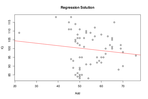
bitmap(file='regressionplot.png')
plot(Y~ X, data=xdf, xlab=V2, ylab=V1, main='Regression Solution')
if(intercept == TRUE) abline(coef(lmxdf), col='red')
if(intercept == FALSE) abline(0.0, coef(lmxdf), col='red')
dev.off()
library(car)
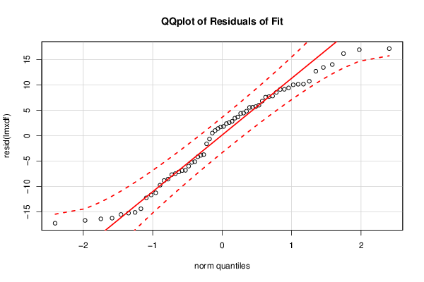
bitmap(file='residualsQQplot.png')
qq.plot(resid(lmxdf), main='QQplot of Residuals of Fit')
dev.off()
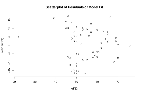
bitmap(file='residualsplot.png')
plot(xdf$X, resid(lmxdf), main='Scatterplot of Residuals of Model Fit')
dev.off()
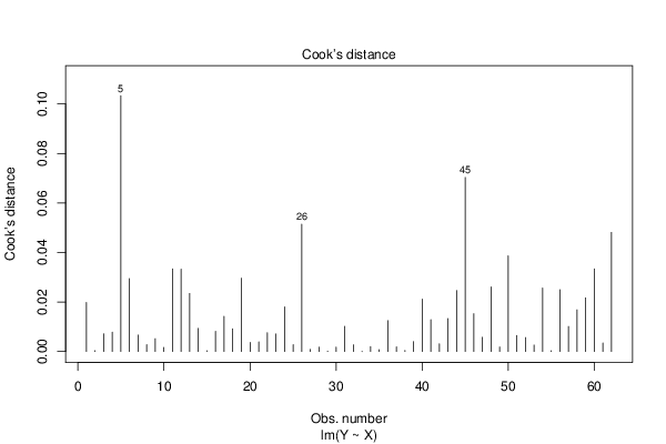
bitmap(file='cooksDistanceLmplot.png')
plot.lm(lmxdf, which=4)
dev.off()

Free Statistics

Description of Statistical Computation

Tree of Dependent Computations

Dataset

Tables (Output of Computation)

Figures (Output of Computation)

Input Parameters & R Code