Free Statistics
of Irreproducible Research!
Description of Statistical Computation | |||||||||||||||||||||
|---|---|---|---|---|---|---|---|---|---|---|---|---|---|---|---|---|---|---|---|---|---|
| Author's title | |||||||||||||||||||||
| Author | *Unverified author* | ||||||||||||||||||||
| R Software Module | rwasp_sdplot.wasp | ||||||||||||||||||||
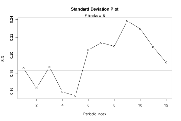
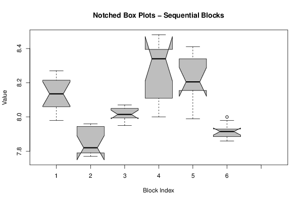
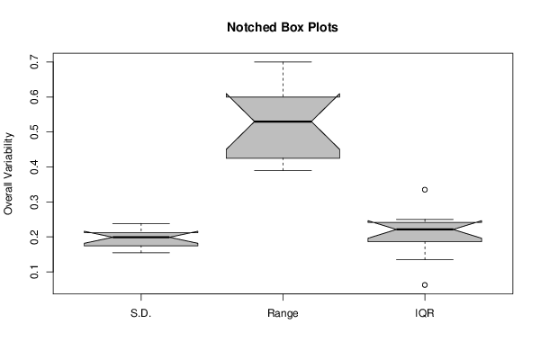
| Title produced by software | Standard Deviation Plot | ||||||||||||||||||||
| Date of computation | Fri, 26 Apr 2013 14:55:07 -0400 | ||||||||||||||||||||
| Cite this page as follows | Statistical Computations at FreeStatistics.org, Office for Research Development and Education, URL https://freestatistics.org/blog/index.php?v=date/2013/Apr/26/t136700257020jtnwp8c6whyqy.htm/, Retrieved Sat, 27 Apr 2024 12:51:41 +0000 | ||||||||||||||||||||
| Statistical Computations at FreeStatistics.org, Office for Research Development and Education, URL https://freestatistics.org/blog/index.php?pk=208403, Retrieved Sat, 27 Apr 2024 12:51:41 +0000 | |||||||||||||||||||||
| QR Codes: | |||||||||||||||||||||
|
| |||||||||||||||||||||
| Original text written by user: | |||||||||||||||||||||
| IsPrivate? | No (this computation is public) | ||||||||||||||||||||
| User-defined keywords | |||||||||||||||||||||
| Estimated Impact | 71 | ||||||||||||||||||||
Tree of Dependent Computations | |||||||||||||||||||||
| Family? (F = Feedback message, R = changed R code, M = changed R Module, P = changed Parameters, D = changed Data) | |||||||||||||||||||||
| - [Standard Deviation Plot] [Spreidingsgrafieken] [2013-04-26 18:55:07] [8907525eeb8291a8059cdce9cf2ca306] [Current] | |||||||||||||||||||||
| Feedback Forum | |||||||||||||||||||||
Post a new message | |||||||||||||||||||||
Dataset | |||||||||||||||||||||
| Dataseries X: | |||||||||||||||||||||
8,27 8,25 8,22 8,21 8,12 8,16 8,15 8,1 8,09 8,02 8,03 7,98 7,95 7,92 7,96 7,96 7,94 7,83 7,77 7,8 7,78 7,78 7,8 7,81 7,95 8,02 7,99 8,01 8,03 8,05 8,05 8,06 8,07 7,99 8 8,01 8 8,09 8,1 8,12 8,29 8,32 8,36 8,38 8,48 8,45 8,41 8,38 8,38 8,34 8,41 8,34 8,22 8,27 8,18 8,19 8,19 8,13 8,06 7,99 8 7,98 7,92 7,93 7,9 7,86 7,88 7,88 7,93 7,91 7,89 7,93 | |||||||||||||||||||||
Tables (Output of Computation) | |||||||||||||||||||||
| |||||||||||||||||||||
Figures (Output of Computation) | |||||||||||||||||||||
Input Parameters & R Code | |||||||||||||||||||||
| Parameters (Session): | |||||||||||||||||||||
| par1 = 12 ; | |||||||||||||||||||||
| Parameters (R input): | |||||||||||||||||||||
| par1 = 12 ; | |||||||||||||||||||||
| R code (references can be found in the software module): | |||||||||||||||||||||
par1 <- as.numeric(par1) | |||||||||||||||||||||