Free Statistics
of Irreproducible Research!
Description of Statistical Computation | |||||||||||||||||||||
|---|---|---|---|---|---|---|---|---|---|---|---|---|---|---|---|---|---|---|---|---|---|
| Author's title | |||||||||||||||||||||
| Author | *Unverified author* | ||||||||||||||||||||
| R Software Module | rwasp_meanplot.wasp | ||||||||||||||||||||
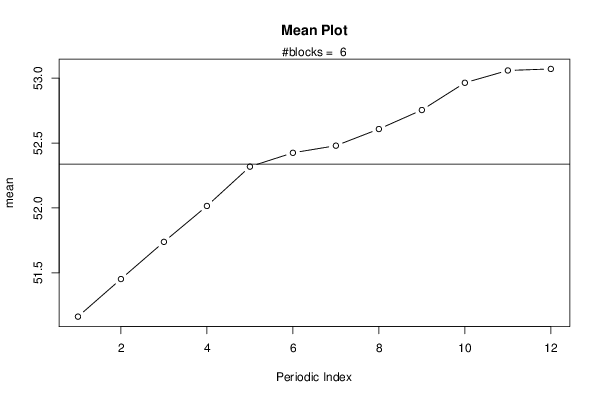
| Title produced by software | Mean Plot | ||||||||||||||||||||
| Date of computation | Wed, 26 Dec 2012 08:44:42 -0500 | ||||||||||||||||||||
| Cite this page as follows | Statistical Computations at FreeStatistics.org, Office for Research Development and Education, URL https://freestatistics.org/blog/index.php?v=date/2012/Dec/26/t13565295161dyhmdlthmdavq0.htm/, Retrieved Sat, 27 Apr 2024 00:19:07 +0000 | ||||||||||||||||||||
| Statistical Computations at FreeStatistics.org, Office for Research Development and Education, URL https://freestatistics.org/blog/index.php?pk=204730, Retrieved Sat, 27 Apr 2024 00:19:07 +0000 | |||||||||||||||||||||
| QR Codes: | |||||||||||||||||||||
|
| |||||||||||||||||||||
| Original text written by user: | |||||||||||||||||||||
| IsPrivate? | No (this computation is public) | ||||||||||||||||||||
| User-defined keywords | |||||||||||||||||||||
| Estimated Impact | 117 | ||||||||||||||||||||
Tree of Dependent Computations | |||||||||||||||||||||
| Family? (F = Feedback message, R = changed R code, M = changed R Module, P = changed Parameters, D = changed Data) | |||||||||||||||||||||
| - [Mean Plot] [uurtarief garage] [2012-12-26 13:44:42] [21b9ad762194a0cf58934491430d34cc] [Current] | |||||||||||||||||||||
| Feedback Forum | |||||||||||||||||||||
Post a new message | |||||||||||||||||||||
Dataset | |||||||||||||||||||||
| Dataseries X: | |||||||||||||||||||||
46,56 46,72 47,01 47,26 47,49 47,51 47,52 47,66 47,71 47,87 48 48 48,05 48,25 48,72 48,94 49,16 49,18 49,25 49,34 49,49 49,57 49,63 49,67 49,7 49,8 50,09 50,49 50,73 51,12 51,15 51,41 51,61 52,06 52,17 52,18 52,19 52,74 53,05 53,38 53,78 53,82 53,88 53,96 54,14 54,2 54,35 54,36 54,39 54,77 54,91 55,06 55,38 55,41 55,47 55,58 55,67 55,97 56,03 56,06 56,08 56,43 56,65 56,96 57,37 57,51 57,61 57,7 57,91 58,12 58,18 58,16 | |||||||||||||||||||||
Tables (Output of Computation) | |||||||||||||||||||||
| |||||||||||||||||||||
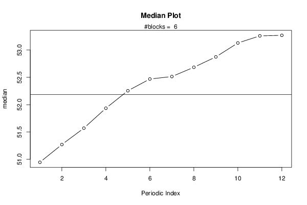
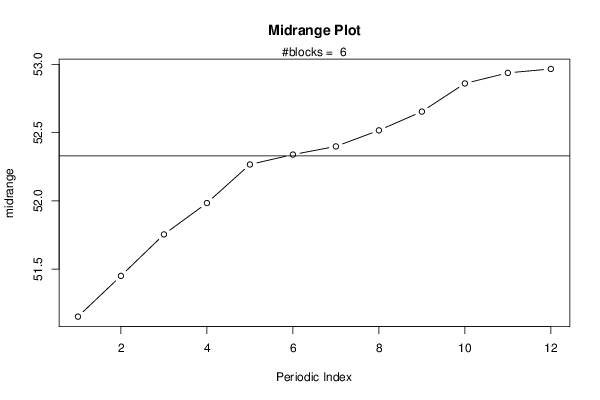
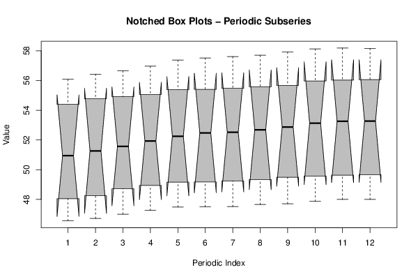
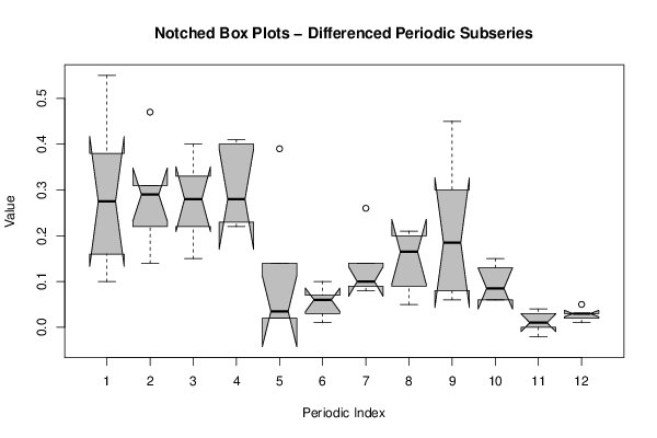
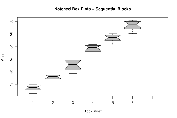
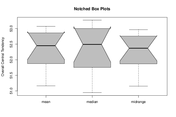
Figures (Output of Computation) | |||||||||||||||||||||
Input Parameters & R Code | |||||||||||||||||||||
| Parameters (Session): | |||||||||||||||||||||
| par1 = 12 ; | |||||||||||||||||||||
| Parameters (R input): | |||||||||||||||||||||
| par1 = 12 ; | |||||||||||||||||||||
| R code (references can be found in the software module): | |||||||||||||||||||||
par1 <- as.numeric(par1) | |||||||||||||||||||||