Free Statistics
of Irreproducible Research!
Description of Statistical Computation | |||||||||||||||||||||
|---|---|---|---|---|---|---|---|---|---|---|---|---|---|---|---|---|---|---|---|---|---|
| Author's title | |||||||||||||||||||||
| Author | *Unverified author* | ||||||||||||||||||||
| R Software Module | rwasp_meanplot.wasp | ||||||||||||||||||||
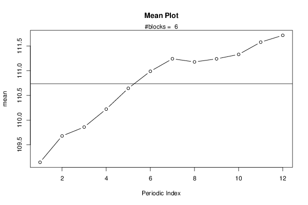
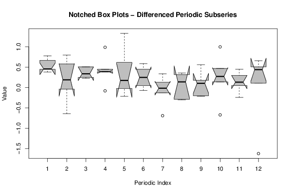
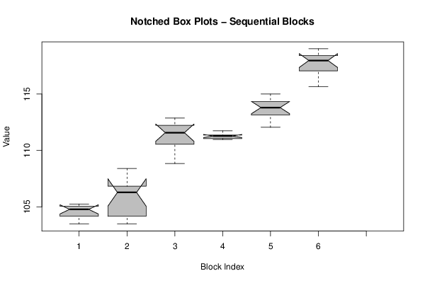
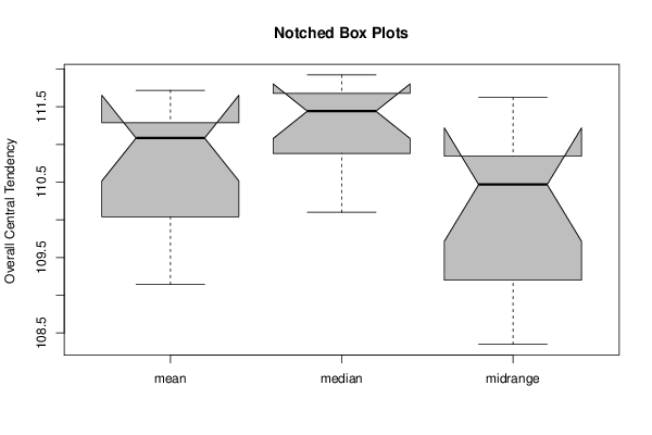
| Title produced by software | Mean Plot | ||||||||||||||||||||
| Date of computation | Wed, 26 Dec 2012 08:02:12 -0500 | ||||||||||||||||||||
| Cite this page as follows | Statistical Computations at FreeStatistics.org, Office for Research Development and Education, URL https://freestatistics.org/blog/index.php?v=date/2012/Dec/26/t1356527045swceshof9c2hsbj.htm/, Retrieved Sat, 20 Apr 2024 14:54:13 +0000 | ||||||||||||||||||||
| Statistical Computations at FreeStatistics.org, Office for Research Development and Education, URL https://freestatistics.org/blog/index.php?pk=204722, Retrieved Sat, 20 Apr 2024 14:54:13 +0000 | |||||||||||||||||||||
| QR Codes: | |||||||||||||||||||||
|
| |||||||||||||||||||||
| Original text written by user: | |||||||||||||||||||||
| IsPrivate? | No (this computation is public) | ||||||||||||||||||||
| User-defined keywords | |||||||||||||||||||||
| Estimated Impact | 127 | ||||||||||||||||||||
Tree of Dependent Computations | |||||||||||||||||||||
| Family? (F = Feedback message, R = changed R code, M = changed R Module, P = changed Parameters, D = changed Data) | |||||||||||||||||||||
| - [Mean Plot] [Consumptieprijsin...] [2012-10-23 05:03:28] [7a81011cbf2af3c6bd3d20955588231b] - R P [Mean Plot] [Consumptieprijsin...] [2012-12-26 13:02:12] [87986ea810528d5717aba44b63d5427b] [Current] | |||||||||||||||||||||
| Feedback Forum | |||||||||||||||||||||
Post a new message | |||||||||||||||||||||
Dataset | |||||||||||||||||||||
| Dataseries X: | |||||||||||||||||||||
103.48 103.93 103.89 104.4 104.79 104.77 105.13 105.26 104.96 104.75 105.01 105.1 103.48 103.93 103.89 104.4 104.79 106.12 106.57 106.44 106.54 107.1 108.1 108.4 108.84 109.62 110.42 110.67 111.66 112.28 112.87 112.18 112.36 112.16 111.49 111.25 111.36 111.74 111.1 111.33 111.25 111.04 110.97 111.31 111.02 111.07 111.36 111.54 112.05 112.52 112.94 113.33 113.78 113.77 113.82 113.89 114.25 114.41 114.55 115 115.66 116.33 116.91 117.2 117.59 117.95 118.09 117.99 118.31 118.49 118.96 119.01 | |||||||||||||||||||||
Tables (Output of Computation) | |||||||||||||||||||||
| |||||||||||||||||||||
Figures (Output of Computation) | |||||||||||||||||||||
Input Parameters & R Code | |||||||||||||||||||||
| Parameters (Session): | |||||||||||||||||||||
| par1 = 12 ; | |||||||||||||||||||||
| Parameters (R input): | |||||||||||||||||||||
| par1 = 12 ; | |||||||||||||||||||||
| R code (references can be found in the software module): | |||||||||||||||||||||
par1 <- as.numeric(par1) | |||||||||||||||||||||