Repository of Reproducible Computations

Free Statistics

of Irreproducible Research!

Author's title

Author

*Unverified author*

R Software Module

rwasp_autocorrelation.wasp

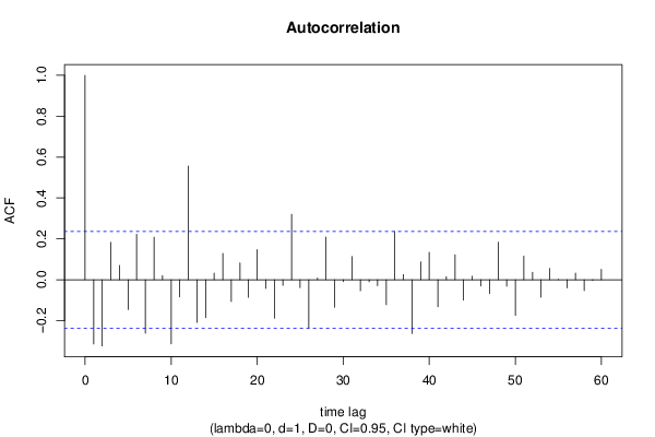
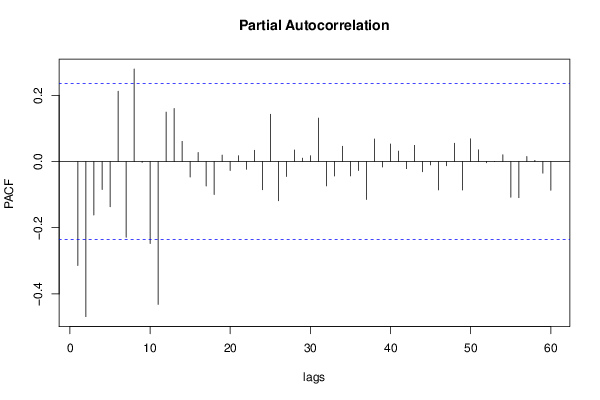
Title produced by software

(Partial) Autocorrelation Function

Date of computation

Sat, 22 Dec 2012 18:48:35 -0500

Cite this page as follows

Statistical Computations at FreeStatistics.org, Office for Research Development and Education, URL https://freestatistics.org/blog/index.php?v=date/2012/Dec/22/t1356220124bxgrmya74f04x2s.htm/, Retrieved Thu, 25 Apr 2024 19:40:27 +0000

Statistical Computations at FreeStatistics.org, Office for Research Development and Education, URL https://freestatistics.org/blog/index.php?pk=204645, Retrieved Thu, 25 Apr 2024 19:40:27 +0000

QR Codes:

Paste this QR Code to cite your computation.

Original text written by user:

IsPrivate?

No (this computation is public)

User-defined keywords

Estimated Impact

105

Family? (F = Feedback message, R = changed R code, M = changed R Module, P = changed Parameters, D = changed Data)

-     [Univariate Explorative Data Analysis] [Run Sequence gebo...] [2008-12-12 13:32:37] [76963dc1903f0f612b6153510a3818cf]
- R  D  [Univariate Explorative Data Analysis] [Run Sequence gebo...] [2008-12-17 12:14:40] [76963dc1903f0f612b6153510a3818cf]
-         [Univariate Explorative Data Analysis] [Run Sequence Plot...] [2008-12-22 18:19:51] [1ce0d16c8f4225c977b42c8fa93bc163]
- RMP       [(Partial) Autocorrelation Function] [Identifying Integ...] [2009-11-22 12:16:10] [b98453cac15ba1066b407e146608df68]
-   PD        [(Partial) Autocorrelation Function] [Identifying Integ...] [2009-12-16 20:15:45] [1eab65e90adf64584b8e6f0da23ff414]
-   P           [(Partial) Autocorrelation Function] [Identifying Integ...] [2009-12-19 16:27:58] [1eab65e90adf64584b8e6f0da23ff414]
- R P               [(Partial) Autocorrelation Function] [] [2012-12-22 23:48:35] [d41d8cd98f00b204e9800998ecf8427e] [Current]

Feedback Forum

Post a new message

Dataseries X:

Download CSV

Histogram

Boxplots

Summary of computational transaction
Raw Input	view raw input (R code)
Raw Output	view raw output of R engine
Computing time	1 seconds
R Server	'Gwilym Jenkins' @ jenkins.wessa.net

\begin{tabular}{lllllllll}
\hline
Summary of computational transaction \tabularnewline
Raw Input & view raw input (R code)  \tabularnewline
Raw Output & view raw output of R engine  \tabularnewline
Computing time & 1 seconds \tabularnewline
R Server & 'Gwilym Jenkins' @ jenkins.wessa.net \tabularnewline
\hline
\end{tabular}
%Source: https://freestatistics.org/blog/index.php?pk=204645&T=0

[TABLE]
[ROW][C]Summary of computational transaction[/C][/ROW]
[ROW][C]Raw Input[/C][C]view raw input (R code) [/C][/ROW]
[ROW][C]Raw Output[/C][C]view raw output of R engine [/C][/ROW]
[ROW][C]Computing time[/C][C]1 seconds[/C][/ROW]
[ROW][C]R Server[/C][C]'Gwilym Jenkins' @ jenkins.wessa.net[/C][/ROW]
[/TABLE]
Source: https://freestatistics.org/blog/index.php?pk=204645&T=0

Globally Unique Identifier (entire table): ba.freestatistics.org/blog/index.php?pk=204645&T=0

As an alternative you can also use a QR Code:

The GUIDs for individual cells are displayed in the table below:

Summary of computational transaction
Raw Input	view raw input (R code)
Raw Output	view raw output of R engine
Computing time	1 seconds
R Server	'Gwilym Jenkins' @ jenkins.wessa.net

Autocorrelation Function
Time lag k	ACF(k)	T-STAT	P-value
1	-0.314148	-2.6095	0.005555
2	-0.32358	-2.6879	0.004503
3	0.182927	1.5195	0.066602
4	0.070394	0.5847	0.280317
5	-0.145933	-1.2122	0.114783
6	0.222223	1.8459	0.034597
7	-0.261373	-2.1711	0.016682
8	0.20849	1.7318	0.043885
9	0.01977	0.1642	0.435018
10	-0.313522	-2.6043	0.005632
11	-0.083361	-0.6925	0.245489
12	0.556139	4.6196	9e-06
13	-0.208599	-1.7328	0.043803
14	-0.185103	-1.5376	0.064362
15	0.032669	0.2714	0.39346
16	0.129106	1.0724	0.14363
17	-0.106636	-0.8858	0.189404
18	0.082502	0.6853	0.247722
19	-0.085734	-0.7122	0.239384
20	0.147934	1.2288	0.111654
21	-0.042398	-0.3522	0.362886
22	-0.187685	-1.559	0.061782
23	-0.027291	-0.2267	0.410666
24	0.320327	2.6608	0.004843
25	-0.03816	-0.317	0.376108
26	-0.236243	-1.9624	0.026876
27	0.008729	0.0725	0.471202
28	0.2086	1.7328	0.043803
29	-0.134744	-1.1193	0.133454
30	-0.008701	-0.0723	0.471296
31	0.113514	0.9429	0.174505
32	-0.053661	-0.4457	0.328591
33	-0.00973	-0.0808	0.46791
34	-0.029231	-0.2428	0.404435
35	-0.121737	-1.0112	0.157722
36	0.23653	1.9648	0.026735
37	0.025118	0.2086	0.417669
38	-0.262985	-2.1845	0.016162
39	0.087458	0.7265	0.235001
40	0.134276	1.1154	0.134279
41	-0.132079	-1.0971	0.138199
42	0.015692	0.1304	0.448334
43	0.121835	1.012	0.157527
44	-0.099509	-0.8266	0.20566
45	0.017122	0.1422	0.443657
46	-0.030072	-0.2498	0.401744
47	-0.066952	-0.5561	0.289955
48	0.183417	1.5236	0.066093
49	-0.03169	-0.2632	0.396576
50	-0.17386	-1.4442	0.076606
51	0.115215	0.957	0.170942
52	0.036465	0.3029	0.381438
53	-0.08513	-0.7071	0.240928
54	0.05515	0.4581	0.324157
55	0.002494	0.0207	0.491766
56	-0.039897	-0.3314	0.37067
57	0.03268	0.2715	0.393423
58	-0.053084	-0.4409	0.330314
59	-0.003375	-0.028	0.488857
60	0.050584	0.4202	0.337828

\begin{tabular}{lllllllll}
\hline
Autocorrelation Function \tabularnewline
Time lag k & ACF(k) & T-STAT & P-value \tabularnewline
1 & -0.314148 & -2.6095 & 0.005555 \tabularnewline
2 & -0.32358 & -2.6879 & 0.004503 \tabularnewline
3 & 0.182927 & 1.5195 & 0.066602 \tabularnewline
4 & 0.070394 & 0.5847 & 0.280317 \tabularnewline
5 & -0.145933 & -1.2122 & 0.114783 \tabularnewline
6 & 0.222223 & 1.8459 & 0.034597 \tabularnewline
7 & -0.261373 & -2.1711 & 0.016682 \tabularnewline
8 & 0.20849 & 1.7318 & 0.043885 \tabularnewline
9 & 0.01977 & 0.1642 & 0.435018 \tabularnewline
10 & -0.313522 & -2.6043 & 0.005632 \tabularnewline
11 & -0.083361 & -0.6925 & 0.245489 \tabularnewline
12 & 0.556139 & 4.6196 & 9e-06 \tabularnewline
13 & -0.208599 & -1.7328 & 0.043803 \tabularnewline
14 & -0.185103 & -1.5376 & 0.064362 \tabularnewline
15 & 0.032669 & 0.2714 & 0.39346 \tabularnewline
16 & 0.129106 & 1.0724 & 0.14363 \tabularnewline
17 & -0.106636 & -0.8858 & 0.189404 \tabularnewline
18 & 0.082502 & 0.6853 & 0.247722 \tabularnewline
19 & -0.085734 & -0.7122 & 0.239384 \tabularnewline
20 & 0.147934 & 1.2288 & 0.111654 \tabularnewline
21 & -0.042398 & -0.3522 & 0.362886 \tabularnewline
22 & -0.187685 & -1.559 & 0.061782 \tabularnewline
23 & -0.027291 & -0.2267 & 0.410666 \tabularnewline
24 & 0.320327 & 2.6608 & 0.004843 \tabularnewline
25 & -0.03816 & -0.317 & 0.376108 \tabularnewline
26 & -0.236243 & -1.9624 & 0.026876 \tabularnewline
27 & 0.008729 & 0.0725 & 0.471202 \tabularnewline
28 & 0.2086 & 1.7328 & 0.043803 \tabularnewline
29 & -0.134744 & -1.1193 & 0.133454 \tabularnewline
30 & -0.008701 & -0.0723 & 0.471296 \tabularnewline
31 & 0.113514 & 0.9429 & 0.174505 \tabularnewline
32 & -0.053661 & -0.4457 & 0.328591 \tabularnewline
33 & -0.00973 & -0.0808 & 0.46791 \tabularnewline
34 & -0.029231 & -0.2428 & 0.404435 \tabularnewline
35 & -0.121737 & -1.0112 & 0.157722 \tabularnewline
36 & 0.23653 & 1.9648 & 0.026735 \tabularnewline
37 & 0.025118 & 0.2086 & 0.417669 \tabularnewline
38 & -0.262985 & -2.1845 & 0.016162 \tabularnewline
39 & 0.087458 & 0.7265 & 0.235001 \tabularnewline
40 & 0.134276 & 1.1154 & 0.134279 \tabularnewline
41 & -0.132079 & -1.0971 & 0.138199 \tabularnewline
42 & 0.015692 & 0.1304 & 0.448334 \tabularnewline
43 & 0.121835 & 1.012 & 0.157527 \tabularnewline
44 & -0.099509 & -0.8266 & 0.20566 \tabularnewline
45 & 0.017122 & 0.1422 & 0.443657 \tabularnewline
46 & -0.030072 & -0.2498 & 0.401744 \tabularnewline
47 & -0.066952 & -0.5561 & 0.289955 \tabularnewline
48 & 0.183417 & 1.5236 & 0.066093 \tabularnewline
49 & -0.03169 & -0.2632 & 0.396576 \tabularnewline
50 & -0.17386 & -1.4442 & 0.076606 \tabularnewline
51 & 0.115215 & 0.957 & 0.170942 \tabularnewline
52 & 0.036465 & 0.3029 & 0.381438 \tabularnewline
53 & -0.08513 & -0.7071 & 0.240928 \tabularnewline
54 & 0.05515 & 0.4581 & 0.324157 \tabularnewline
55 & 0.002494 & 0.0207 & 0.491766 \tabularnewline
56 & -0.039897 & -0.3314 & 0.37067 \tabularnewline
57 & 0.03268 & 0.2715 & 0.393423 \tabularnewline
58 & -0.053084 & -0.4409 & 0.330314 \tabularnewline
59 & -0.003375 & -0.028 & 0.488857 \tabularnewline
60 & 0.050584 & 0.4202 & 0.337828 \tabularnewline
\hline
\end{tabular}
%Source: https://freestatistics.org/blog/index.php?pk=204645&T=1

[TABLE]
[ROW][C]Autocorrelation Function[/C][/ROW]
[ROW][C]Time lag k[/C][C]ACF(k)[/C][C]T-STAT[/C][C]P-value[/C][/ROW]
[ROW][C]1[/C][C]-0.314148[/C][C]-2.6095[/C][C]0.005555[/C][/ROW]
[ROW][C]2[/C][C]-0.32358[/C][C]-2.6879[/C][C]0.004503[/C][/ROW]
[ROW][C]3[/C][C]0.182927[/C][C]1.5195[/C][C]0.066602[/C][/ROW]
[ROW][C]4[/C][C]0.070394[/C][C]0.5847[/C][C]0.280317[/C][/ROW]
[ROW][C]5[/C][C]-0.145933[/C][C]-1.2122[/C][C]0.114783[/C][/ROW]
[ROW][C]6[/C][C]0.222223[/C][C]1.8459[/C][C]0.034597[/C][/ROW]
[ROW][C]7[/C][C]-0.261373[/C][C]-2.1711[/C][C]0.016682[/C][/ROW]
[ROW][C]8[/C][C]0.20849[/C][C]1.7318[/C][C]0.043885[/C][/ROW]
[ROW][C]9[/C][C]0.01977[/C][C]0.1642[/C][C]0.435018[/C][/ROW]
[ROW][C]10[/C][C]-0.313522[/C][C]-2.6043[/C][C]0.005632[/C][/ROW]
[ROW][C]11[/C][C]-0.083361[/C][C]-0.6925[/C][C]0.245489[/C][/ROW]
[ROW][C]12[/C][C]0.556139[/C][C]4.6196[/C][C]9e-06[/C][/ROW]
[ROW][C]13[/C][C]-0.208599[/C][C]-1.7328[/C][C]0.043803[/C][/ROW]
[ROW][C]14[/C][C]-0.185103[/C][C]-1.5376[/C][C]0.064362[/C][/ROW]
[ROW][C]15[/C][C]0.032669[/C][C]0.2714[/C][C]0.39346[/C][/ROW]
[ROW][C]16[/C][C]0.129106[/C][C]1.0724[/C][C]0.14363[/C][/ROW]
[ROW][C]17[/C][C]-0.106636[/C][C]-0.8858[/C][C]0.189404[/C][/ROW]
[ROW][C]18[/C][C]0.082502[/C][C]0.6853[/C][C]0.247722[/C][/ROW]
[ROW][C]19[/C][C]-0.085734[/C][C]-0.7122[/C][C]0.239384[/C][/ROW]
[ROW][C]20[/C][C]0.147934[/C][C]1.2288[/C][C]0.111654[/C][/ROW]
[ROW][C]21[/C][C]-0.042398[/C][C]-0.3522[/C][C]0.362886[/C][/ROW]
[ROW][C]22[/C][C]-0.187685[/C][C]-1.559[/C][C]0.061782[/C][/ROW]
[ROW][C]23[/C][C]-0.027291[/C][C]-0.2267[/C][C]0.410666[/C][/ROW]
[ROW][C]24[/C][C]0.320327[/C][C]2.6608[/C][C]0.004843[/C][/ROW]
[ROW][C]25[/C][C]-0.03816[/C][C]-0.317[/C][C]0.376108[/C][/ROW]
[ROW][C]26[/C][C]-0.236243[/C][C]-1.9624[/C][C]0.026876[/C][/ROW]
[ROW][C]27[/C][C]0.008729[/C][C]0.0725[/C][C]0.471202[/C][/ROW]
[ROW][C]28[/C][C]0.2086[/C][C]1.7328[/C][C]0.043803[/C][/ROW]
[ROW][C]29[/C][C]-0.134744[/C][C]-1.1193[/C][C]0.133454[/C][/ROW]
[ROW][C]30[/C][C]-0.008701[/C][C]-0.0723[/C][C]0.471296[/C][/ROW]
[ROW][C]31[/C][C]0.113514[/C][C]0.9429[/C][C]0.174505[/C][/ROW]
[ROW][C]32[/C][C]-0.053661[/C][C]-0.4457[/C][C]0.328591[/C][/ROW]
[ROW][C]33[/C][C]-0.00973[/C][C]-0.0808[/C][C]0.46791[/C][/ROW]
[ROW][C]34[/C][C]-0.029231[/C][C]-0.2428[/C][C]0.404435[/C][/ROW]
[ROW][C]35[/C][C]-0.121737[/C][C]-1.0112[/C][C]0.157722[/C][/ROW]
[ROW][C]36[/C][C]0.23653[/C][C]1.9648[/C][C]0.026735[/C][/ROW]
[ROW][C]37[/C][C]0.025118[/C][C]0.2086[/C][C]0.417669[/C][/ROW]
[ROW][C]38[/C][C]-0.262985[/C][C]-2.1845[/C][C]0.016162[/C][/ROW]
[ROW][C]39[/C][C]0.087458[/C][C]0.7265[/C][C]0.235001[/C][/ROW]
[ROW][C]40[/C][C]0.134276[/C][C]1.1154[/C][C]0.134279[/C][/ROW]
[ROW][C]41[/C][C]-0.132079[/C][C]-1.0971[/C][C]0.138199[/C][/ROW]
[ROW][C]42[/C][C]0.015692[/C][C]0.1304[/C][C]0.448334[/C][/ROW]
[ROW][C]43[/C][C]0.121835[/C][C]1.012[/C][C]0.157527[/C][/ROW]
[ROW][C]44[/C][C]-0.099509[/C][C]-0.8266[/C][C]0.20566[/C][/ROW]
[ROW][C]45[/C][C]0.017122[/C][C]0.1422[/C][C]0.443657[/C][/ROW]
[ROW][C]46[/C][C]-0.030072[/C][C]-0.2498[/C][C]0.401744[/C][/ROW]
[ROW][C]47[/C][C]-0.066952[/C][C]-0.5561[/C][C]0.289955[/C][/ROW]
[ROW][C]48[/C][C]0.183417[/C][C]1.5236[/C][C]0.066093[/C][/ROW]
[ROW][C]49[/C][C]-0.03169[/C][C]-0.2632[/C][C]0.396576[/C][/ROW]
[ROW][C]50[/C][C]-0.17386[/C][C]-1.4442[/C][C]0.076606[/C][/ROW]
[ROW][C]51[/C][C]0.115215[/C][C]0.957[/C][C]0.170942[/C][/ROW]
[ROW][C]52[/C][C]0.036465[/C][C]0.3029[/C][C]0.381438[/C][/ROW]
[ROW][C]53[/C][C]-0.08513[/C][C]-0.7071[/C][C]0.240928[/C][/ROW]
[ROW][C]54[/C][C]0.05515[/C][C]0.4581[/C][C]0.324157[/C][/ROW]
[ROW][C]55[/C][C]0.002494[/C][C]0.0207[/C][C]0.491766[/C][/ROW]
[ROW][C]56[/C][C]-0.039897[/C][C]-0.3314[/C][C]0.37067[/C][/ROW]
[ROW][C]57[/C][C]0.03268[/C][C]0.2715[/C][C]0.393423[/C][/ROW]
[ROW][C]58[/C][C]-0.053084[/C][C]-0.4409[/C][C]0.330314[/C][/ROW]
[ROW][C]59[/C][C]-0.003375[/C][C]-0.028[/C][C]0.488857[/C][/ROW]
[ROW][C]60[/C][C]0.050584[/C][C]0.4202[/C][C]0.337828[/C][/ROW]
[/TABLE]
Source: https://freestatistics.org/blog/index.php?pk=204645&T=1

Globally Unique Identifier (entire table): ba.freestatistics.org/blog/index.php?pk=204645&T=1

As an alternative you can also use a QR Code:

The GUIDs for individual cells are displayed in the table below:

Autocorrelation Function
Time lag k	ACF(k)	T-STAT	P-value
1	-0.314148	-2.6095	0.005555
2	-0.32358	-2.6879	0.004503
3	0.182927	1.5195	0.066602
4	0.070394	0.5847	0.280317
5	-0.145933	-1.2122	0.114783
6	0.222223	1.8459	0.034597
7	-0.261373	-2.1711	0.016682
8	0.20849	1.7318	0.043885
9	0.01977	0.1642	0.435018
10	-0.313522	-2.6043	0.005632
11	-0.083361	-0.6925	0.245489
12	0.556139	4.6196	9e-06
13	-0.208599	-1.7328	0.043803
14	-0.185103	-1.5376	0.064362
15	0.032669	0.2714	0.39346
16	0.129106	1.0724	0.14363
17	-0.106636	-0.8858	0.189404
18	0.082502	0.6853	0.247722
19	-0.085734	-0.7122	0.239384
20	0.147934	1.2288	0.111654
21	-0.042398	-0.3522	0.362886
22	-0.187685	-1.559	0.061782
23	-0.027291	-0.2267	0.410666
24	0.320327	2.6608	0.004843
25	-0.03816	-0.317	0.376108
26	-0.236243	-1.9624	0.026876
27	0.008729	0.0725	0.471202
28	0.2086	1.7328	0.043803
29	-0.134744	-1.1193	0.133454
30	-0.008701	-0.0723	0.471296
31	0.113514	0.9429	0.174505
32	-0.053661	-0.4457	0.328591
33	-0.00973	-0.0808	0.46791
34	-0.029231	-0.2428	0.404435
35	-0.121737	-1.0112	0.157722
36	0.23653	1.9648	0.026735
37	0.025118	0.2086	0.417669
38	-0.262985	-2.1845	0.016162
39	0.087458	0.7265	0.235001
40	0.134276	1.1154	0.134279
41	-0.132079	-1.0971	0.138199
42	0.015692	0.1304	0.448334
43	0.121835	1.012	0.157527
44	-0.099509	-0.8266	0.20566
45	0.017122	0.1422	0.443657
46	-0.030072	-0.2498	0.401744
47	-0.066952	-0.5561	0.289955
48	0.183417	1.5236	0.066093
49	-0.03169	-0.2632	0.396576
50	-0.17386	-1.4442	0.076606
51	0.115215	0.957	0.170942
52	0.036465	0.3029	0.381438
53	-0.08513	-0.7071	0.240928
54	0.05515	0.4581	0.324157
55	0.002494	0.0207	0.491766
56	-0.039897	-0.3314	0.37067
57	0.03268	0.2715	0.393423
58	-0.053084	-0.4409	0.330314
59	-0.003375	-0.028	0.488857
60	0.050584	0.4202	0.337828

Partial Autocorrelation Function
Time lag k	PACF(k)	T-STAT	P-value
1	-0.314148	-2.6095	0.005555
2	-0.468505	-3.8917	0.000113
3	-0.161384	-1.3406	0.092231
4	-0.084323	-0.7004	0.243003
5	-0.136477	-1.1337	0.13043
6	0.212189	1.7626	0.041201
7	-0.228647	-1.8993	0.030854
8	0.27956	2.3222	0.01159
9	-0.002697	-0.0224	0.491096
10	-0.247793	-2.0583	0.021669
11	-0.431479	-3.5841	0.000313
12	0.149115	1.2386	0.109837
13	0.160257	1.3312	0.093754
14	0.06084	0.5054	0.307452
15	-0.046554	-0.3867	0.350083
16	0.027414	0.2277	0.410271
17	-0.073817	-0.6132	0.27089
18	-0.099803	-0.829	0.204974
19	0.019316	0.1605	0.436498
20	-0.026949	-0.2239	0.411766
21	0.017585	0.1461	0.442144
22	-0.023428	-0.1946	0.423135
23	0.034137	0.2836	0.388798
24	-0.085218	-0.7079	0.240705
25	0.142691	1.1853	0.119986
26	-0.118723	-0.9862	0.163743
27	-0.045162	-0.3751	0.354353
28	0.034715	0.2884	0.386966
29	0.010157	0.0844	0.466502
30	0.017384	0.1444	0.442801
31	0.131079	1.0888	0.140011
32	-0.073662	-0.6119	0.271314
33	-0.043596	-0.3621	0.35918
34	0.046211	0.3839	0.351131
35	-0.043389	-0.3604	0.35982
36	-0.027325	-0.227	0.410556
37	-0.114914	-0.9545	0.171569
38	0.068023	0.565	0.286939
39	-0.016697	-0.1387	0.445047
40	0.052844	0.439	0.331034
41	0.031485	0.2615	0.397231
42	-0.0216	-0.1794	0.429066
43	0.048712	0.4046	0.343501
44	-0.030883	-0.2565	0.399151
45	-0.010211	-0.0848	0.466327
46	-0.085594	-0.711	0.239742
47	-0.012617	-0.1048	0.458417
48	0.055399	0.4602	0.323418
49	-0.086175	-0.7158	0.238258
50	0.068521	0.5692	0.285542
51	0.035173	0.2922	0.385516
52	-0.00353	-0.0293	0.488345
53	-3e-06	0	0.49999
54	0.020626	0.1713	0.432231
55	-0.108161	-0.8985	0.186034
56	-0.109061	-0.9059	0.184063
57	0.015047	0.125	0.450447
58	0.003493	0.029	0.488469
59	-0.035044	-0.2911	0.385924
60	-0.086971	-0.7224	0.236234

\begin{tabular}{lllllllll}
\hline
Partial Autocorrelation Function \tabularnewline
Time lag k & PACF(k) & T-STAT & P-value \tabularnewline
1 & -0.314148 & -2.6095 & 0.005555 \tabularnewline
2 & -0.468505 & -3.8917 & 0.000113 \tabularnewline
3 & -0.161384 & -1.3406 & 0.092231 \tabularnewline
4 & -0.084323 & -0.7004 & 0.243003 \tabularnewline
5 & -0.136477 & -1.1337 & 0.13043 \tabularnewline
6 & 0.212189 & 1.7626 & 0.041201 \tabularnewline
7 & -0.228647 & -1.8993 & 0.030854 \tabularnewline
8 & 0.27956 & 2.3222 & 0.01159 \tabularnewline
9 & -0.002697 & -0.0224 & 0.491096 \tabularnewline
10 & -0.247793 & -2.0583 & 0.021669 \tabularnewline
11 & -0.431479 & -3.5841 & 0.000313 \tabularnewline
12 & 0.149115 & 1.2386 & 0.109837 \tabularnewline
13 & 0.160257 & 1.3312 & 0.093754 \tabularnewline
14 & 0.06084 & 0.5054 & 0.307452 \tabularnewline
15 & -0.046554 & -0.3867 & 0.350083 \tabularnewline
16 & 0.027414 & 0.2277 & 0.410271 \tabularnewline
17 & -0.073817 & -0.6132 & 0.27089 \tabularnewline
18 & -0.099803 & -0.829 & 0.204974 \tabularnewline
19 & 0.019316 & 0.1605 & 0.436498 \tabularnewline
20 & -0.026949 & -0.2239 & 0.411766 \tabularnewline
21 & 0.017585 & 0.1461 & 0.442144 \tabularnewline
22 & -0.023428 & -0.1946 & 0.423135 \tabularnewline
23 & 0.034137 & 0.2836 & 0.388798 \tabularnewline
24 & -0.085218 & -0.7079 & 0.240705 \tabularnewline
25 & 0.142691 & 1.1853 & 0.119986 \tabularnewline
26 & -0.118723 & -0.9862 & 0.163743 \tabularnewline
27 & -0.045162 & -0.3751 & 0.354353 \tabularnewline
28 & 0.034715 & 0.2884 & 0.386966 \tabularnewline
29 & 0.010157 & 0.0844 & 0.466502 \tabularnewline
30 & 0.017384 & 0.1444 & 0.442801 \tabularnewline
31 & 0.131079 & 1.0888 & 0.140011 \tabularnewline
32 & -0.073662 & -0.6119 & 0.271314 \tabularnewline
33 & -0.043596 & -0.3621 & 0.35918 \tabularnewline
34 & 0.046211 & 0.3839 & 0.351131 \tabularnewline
35 & -0.043389 & -0.3604 & 0.35982 \tabularnewline
36 & -0.027325 & -0.227 & 0.410556 \tabularnewline
37 & -0.114914 & -0.9545 & 0.171569 \tabularnewline
38 & 0.068023 & 0.565 & 0.286939 \tabularnewline
39 & -0.016697 & -0.1387 & 0.445047 \tabularnewline
40 & 0.052844 & 0.439 & 0.331034 \tabularnewline
41 & 0.031485 & 0.2615 & 0.397231 \tabularnewline
42 & -0.0216 & -0.1794 & 0.429066 \tabularnewline
43 & 0.048712 & 0.4046 & 0.343501 \tabularnewline
44 & -0.030883 & -0.2565 & 0.399151 \tabularnewline
45 & -0.010211 & -0.0848 & 0.466327 \tabularnewline
46 & -0.085594 & -0.711 & 0.239742 \tabularnewline
47 & -0.012617 & -0.1048 & 0.458417 \tabularnewline
48 & 0.055399 & 0.4602 & 0.323418 \tabularnewline
49 & -0.086175 & -0.7158 & 0.238258 \tabularnewline
50 & 0.068521 & 0.5692 & 0.285542 \tabularnewline
51 & 0.035173 & 0.2922 & 0.385516 \tabularnewline
52 & -0.00353 & -0.0293 & 0.488345 \tabularnewline
53 & -3e-06 & 0 & 0.49999 \tabularnewline
54 & 0.020626 & 0.1713 & 0.432231 \tabularnewline
55 & -0.108161 & -0.8985 & 0.186034 \tabularnewline
56 & -0.109061 & -0.9059 & 0.184063 \tabularnewline
57 & 0.015047 & 0.125 & 0.450447 \tabularnewline
58 & 0.003493 & 0.029 & 0.488469 \tabularnewline
59 & -0.035044 & -0.2911 & 0.385924 \tabularnewline
60 & -0.086971 & -0.7224 & 0.236234 \tabularnewline
\hline
\end{tabular}
%Source: https://freestatistics.org/blog/index.php?pk=204645&T=2

[TABLE]
[ROW][C]Partial Autocorrelation Function[/C][/ROW]
[ROW][C]Time lag k[/C][C]PACF(k)[/C][C]T-STAT[/C][C]P-value[/C][/ROW]
[ROW][C]1[/C][C]-0.314148[/C][C]-2.6095[/C][C]0.005555[/C][/ROW]
[ROW][C]2[/C][C]-0.468505[/C][C]-3.8917[/C][C]0.000113[/C][/ROW]
[ROW][C]3[/C][C]-0.161384[/C][C]-1.3406[/C][C]0.092231[/C][/ROW]
[ROW][C]4[/C][C]-0.084323[/C][C]-0.7004[/C][C]0.243003[/C][/ROW]
[ROW][C]5[/C][C]-0.136477[/C][C]-1.1337[/C][C]0.13043[/C][/ROW]
[ROW][C]6[/C][C]0.212189[/C][C]1.7626[/C][C]0.041201[/C][/ROW]
[ROW][C]7[/C][C]-0.228647[/C][C]-1.8993[/C][C]0.030854[/C][/ROW]
[ROW][C]8[/C][C]0.27956[/C][C]2.3222[/C][C]0.01159[/C][/ROW]
[ROW][C]9[/C][C]-0.002697[/C][C]-0.0224[/C][C]0.491096[/C][/ROW]
[ROW][C]10[/C][C]-0.247793[/C][C]-2.0583[/C][C]0.021669[/C][/ROW]
[ROW][C]11[/C][C]-0.431479[/C][C]-3.5841[/C][C]0.000313[/C][/ROW]
[ROW][C]12[/C][C]0.149115[/C][C]1.2386[/C][C]0.109837[/C][/ROW]
[ROW][C]13[/C][C]0.160257[/C][C]1.3312[/C][C]0.093754[/C][/ROW]
[ROW][C]14[/C][C]0.06084[/C][C]0.5054[/C][C]0.307452[/C][/ROW]
[ROW][C]15[/C][C]-0.046554[/C][C]-0.3867[/C][C]0.350083[/C][/ROW]
[ROW][C]16[/C][C]0.027414[/C][C]0.2277[/C][C]0.410271[/C][/ROW]
[ROW][C]17[/C][C]-0.073817[/C][C]-0.6132[/C][C]0.27089[/C][/ROW]
[ROW][C]18[/C][C]-0.099803[/C][C]-0.829[/C][C]0.204974[/C][/ROW]
[ROW][C]19[/C][C]0.019316[/C][C]0.1605[/C][C]0.436498[/C][/ROW]
[ROW][C]20[/C][C]-0.026949[/C][C]-0.2239[/C][C]0.411766[/C][/ROW]
[ROW][C]21[/C][C]0.017585[/C][C]0.1461[/C][C]0.442144[/C][/ROW]
[ROW][C]22[/C][C]-0.023428[/C][C]-0.1946[/C][C]0.423135[/C][/ROW]
[ROW][C]23[/C][C]0.034137[/C][C]0.2836[/C][C]0.388798[/C][/ROW]
[ROW][C]24[/C][C]-0.085218[/C][C]-0.7079[/C][C]0.240705[/C][/ROW]
[ROW][C]25[/C][C]0.142691[/C][C]1.1853[/C][C]0.119986[/C][/ROW]
[ROW][C]26[/C][C]-0.118723[/C][C]-0.9862[/C][C]0.163743[/C][/ROW]
[ROW][C]27[/C][C]-0.045162[/C][C]-0.3751[/C][C]0.354353[/C][/ROW]
[ROW][C]28[/C][C]0.034715[/C][C]0.2884[/C][C]0.386966[/C][/ROW]
[ROW][C]29[/C][C]0.010157[/C][C]0.0844[/C][C]0.466502[/C][/ROW]
[ROW][C]30[/C][C]0.017384[/C][C]0.1444[/C][C]0.442801[/C][/ROW]
[ROW][C]31[/C][C]0.131079[/C][C]1.0888[/C][C]0.140011[/C][/ROW]
[ROW][C]32[/C][C]-0.073662[/C][C]-0.6119[/C][C]0.271314[/C][/ROW]
[ROW][C]33[/C][C]-0.043596[/C][C]-0.3621[/C][C]0.35918[/C][/ROW]
[ROW][C]34[/C][C]0.046211[/C][C]0.3839[/C][C]0.351131[/C][/ROW]
[ROW][C]35[/C][C]-0.043389[/C][C]-0.3604[/C][C]0.35982[/C][/ROW]
[ROW][C]36[/C][C]-0.027325[/C][C]-0.227[/C][C]0.410556[/C][/ROW]
[ROW][C]37[/C][C]-0.114914[/C][C]-0.9545[/C][C]0.171569[/C][/ROW]
[ROW][C]38[/C][C]0.068023[/C][C]0.565[/C][C]0.286939[/C][/ROW]
[ROW][C]39[/C][C]-0.016697[/C][C]-0.1387[/C][C]0.445047[/C][/ROW]
[ROW][C]40[/C][C]0.052844[/C][C]0.439[/C][C]0.331034[/C][/ROW]
[ROW][C]41[/C][C]0.031485[/C][C]0.2615[/C][C]0.397231[/C][/ROW]
[ROW][C]42[/C][C]-0.0216[/C][C]-0.1794[/C][C]0.429066[/C][/ROW]
[ROW][C]43[/C][C]0.048712[/C][C]0.4046[/C][C]0.343501[/C][/ROW]
[ROW][C]44[/C][C]-0.030883[/C][C]-0.2565[/C][C]0.399151[/C][/ROW]
[ROW][C]45[/C][C]-0.010211[/C][C]-0.0848[/C][C]0.466327[/C][/ROW]
[ROW][C]46[/C][C]-0.085594[/C][C]-0.711[/C][C]0.239742[/C][/ROW]
[ROW][C]47[/C][C]-0.012617[/C][C]-0.1048[/C][C]0.458417[/C][/ROW]
[ROW][C]48[/C][C]0.055399[/C][C]0.4602[/C][C]0.323418[/C][/ROW]
[ROW][C]49[/C][C]-0.086175[/C][C]-0.7158[/C][C]0.238258[/C][/ROW]
[ROW][C]50[/C][C]0.068521[/C][C]0.5692[/C][C]0.285542[/C][/ROW]
[ROW][C]51[/C][C]0.035173[/C][C]0.2922[/C][C]0.385516[/C][/ROW]
[ROW][C]52[/C][C]-0.00353[/C][C]-0.0293[/C][C]0.488345[/C][/ROW]
[ROW][C]53[/C][C]-3e-06[/C][C]0[/C][C]0.49999[/C][/ROW]
[ROW][C]54[/C][C]0.020626[/C][C]0.1713[/C][C]0.432231[/C][/ROW]
[ROW][C]55[/C][C]-0.108161[/C][C]-0.8985[/C][C]0.186034[/C][/ROW]
[ROW][C]56[/C][C]-0.109061[/C][C]-0.9059[/C][C]0.184063[/C][/ROW]
[ROW][C]57[/C][C]0.015047[/C][C]0.125[/C][C]0.450447[/C][/ROW]
[ROW][C]58[/C][C]0.003493[/C][C]0.029[/C][C]0.488469[/C][/ROW]
[ROW][C]59[/C][C]-0.035044[/C][C]-0.2911[/C][C]0.385924[/C][/ROW]
[ROW][C]60[/C][C]-0.086971[/C][C]-0.7224[/C][C]0.236234[/C][/ROW]
[/TABLE]
Source: https://freestatistics.org/blog/index.php?pk=204645&T=2

Globally Unique Identifier (entire table): ba.freestatistics.org/blog/index.php?pk=204645&T=2

As an alternative you can also use a QR Code:

The GUIDs for individual cells are displayed in the table below:

Partial Autocorrelation Function
Time lag k	PACF(k)	T-STAT	P-value
1	-0.314148	-2.6095	0.005555
2	-0.468505	-3.8917	0.000113
3	-0.161384	-1.3406	0.092231
4	-0.084323	-0.7004	0.243003
5	-0.136477	-1.1337	0.13043
6	0.212189	1.7626	0.041201
7	-0.228647	-1.8993	0.030854
8	0.27956	2.3222	0.01159
9	-0.002697	-0.0224	0.491096
10	-0.247793	-2.0583	0.021669
11	-0.431479	-3.5841	0.000313
12	0.149115	1.2386	0.109837
13	0.160257	1.3312	0.093754
14	0.06084	0.5054	0.307452
15	-0.046554	-0.3867	0.350083
16	0.027414	0.2277	0.410271
17	-0.073817	-0.6132	0.27089
18	-0.099803	-0.829	0.204974
19	0.019316	0.1605	0.436498
20	-0.026949	-0.2239	0.411766
21	0.017585	0.1461	0.442144
22	-0.023428	-0.1946	0.423135
23	0.034137	0.2836	0.388798
24	-0.085218	-0.7079	0.240705
25	0.142691	1.1853	0.119986
26	-0.118723	-0.9862	0.163743
27	-0.045162	-0.3751	0.354353
28	0.034715	0.2884	0.386966
29	0.010157	0.0844	0.466502
30	0.017384	0.1444	0.442801
31	0.131079	1.0888	0.140011
32	-0.073662	-0.6119	0.271314
33	-0.043596	-0.3621	0.35918
34	0.046211	0.3839	0.351131
35	-0.043389	-0.3604	0.35982
36	-0.027325	-0.227	0.410556
37	-0.114914	-0.9545	0.171569
38	0.068023	0.565	0.286939
39	-0.016697	-0.1387	0.445047
40	0.052844	0.439	0.331034
41	0.031485	0.2615	0.397231
42	-0.0216	-0.1794	0.429066
43	0.048712	0.4046	0.343501
44	-0.030883	-0.2565	0.399151
45	-0.010211	-0.0848	0.466327
46	-0.085594	-0.711	0.239742
47	-0.012617	-0.1048	0.458417
48	0.055399	0.4602	0.323418
49	-0.086175	-0.7158	0.238258
50	0.068521	0.5692	0.285542
51	0.035173	0.2922	0.385516
52	-0.00353	-0.0293	0.488345
53	-3e-06	0	0.49999
54	0.020626	0.1713	0.432231
55	-0.108161	-0.8985	0.186034
56	-0.109061	-0.9059	0.184063
57	0.015047	0.125	0.450447
58	0.003493	0.029	0.488469
59	-0.035044	-0.2911	0.385924
60	-0.086971	-0.7224	0.236234

Figure 1

PNG link

Postscript link

PDF link

Figure 2

PNG link

Postscript link

PDF link

Parameters (Session):

par1 = 50 ; par2 = 36 ;

Parameters (R input):

par1 = 60 ; par2 = 0.0 ; par3 = 1 ; par4 = 0 ; par5 = 12 ; par6 = White Noise ; par7 = 0.95 ; par8 = ;

R code (references can be found in the software module):

if (par1 == 'Default') {
par1 = 10*log10(length(x))
} else {
par1 <- as.numeric(par1)
}
par2 <- as.numeric(par2)
par3 <- as.numeric(par3)
par4 <- as.numeric(par4)
par5 <- as.numeric(par5)
if (par6 == 'White Noise') par6 <- 'white' else par6 <- 'ma'
par7 <- as.numeric(par7)
if (par2 == 0) {
x <- log(x)
} else {
x <- (x ^ par2 - 1) / par2
}
if (par3 > 0) x <- diff(x,lag=1,difference=par3)
if (par4 > 0) x <- diff(x,lag=par5,difference=par4)
bitmap(file='pic1.png')
racf <- acf(x, par1, main='Autocorrelation', xlab='time lag', ylab='ACF', ci.type=par6, ci=par7, sub=paste('(lambda=',par2,', d=',par3,', D=',par4,', CI=', par7, ', CI type=',par6,')',sep=''))
dev.off()
bitmap(file='pic2.png')
rpacf <- pacf(x,par1,main='Partial Autocorrelation',xlab='lags',ylab='PACF')
dev.off()
(myacf <- c(racf$acf))
(mypacf <- c(rpacf$acf))
lengthx <- length(x)
sqrtn <- sqrt(lengthx)
load(file='createtable')
a<-table.start()
a<-table.row.start(a)
a<-table.element(a,'Autocorrelation Function',4,TRUE)
a<-table.row.end(a)
a<-table.row.start(a)
a<-table.element(a,'Time lag k',header=TRUE)
a<-table.element(a,hyperlink('basics.htm','ACF(k)','click here for more information about the Autocorrelation Function'),header=TRUE)
a<-table.element(a,'T-STAT',header=TRUE)
a<-table.element(a,'P-value',header=TRUE)
a<-table.row.end(a)
for (i in 2:(par1+1)) {
a<-table.row.start(a)
a<-table.element(a,i-1,header=TRUE)
a<-table.element(a,round(myacf[i],6))
mytstat <- myacf[i]*sqrtn
a<-table.element(a,round(mytstat,4))
a<-table.element(a,round(1-pt(abs(mytstat),lengthx),6))
a<-table.row.end(a)
}
a<-table.end(a)
table.save(a,file='mytable.tab')
a<-table.start()
a<-table.row.start(a)
a<-table.element(a,'Partial Autocorrelation Function',4,TRUE)
a<-table.row.end(a)
a<-table.row.start(a)
a<-table.element(a,'Time lag k',header=TRUE)
a<-table.element(a,hyperlink('basics.htm','PACF(k)','click here for more information about the Partial Autocorrelation Function'),header=TRUE)
a<-table.element(a,'T-STAT',header=TRUE)
a<-table.element(a,'P-value',header=TRUE)
a<-table.row.end(a)
for (i in 1:par1) {
a<-table.row.start(a)
a<-table.element(a,i,header=TRUE)
a<-table.element(a,round(mypacf[i],6))
mytstat <- mypacf[i]*sqrtn
a<-table.element(a,round(mytstat,4))
a<-table.element(a,round(1-pt(abs(mytstat),lengthx),6))
a<-table.row.end(a)
}
a<-table.end(a)
table.save(a,file='mytable1.tab')

Free Statistics

Description of Statistical Computation

Tree of Dependent Computations

Dataset

Tables (Output of Computation)

Figures (Output of Computation)

Input Parameters & R Code