Free Statistics
of Irreproducible Research!
Description of Statistical Computation | |||||||||||||||||||||||||||||||||||||||||||||||||||||||||||||||||||||||||||||||||||||||||||||||||||||||||||||||||||||||||||||||||||||||||||||||||||||||||||||||||||||||||||||||||||||||||||||||||||||||||||||||||||||||||||||||||||||||||||||||||||||||||||||||||||||||||||
|---|---|---|---|---|---|---|---|---|---|---|---|---|---|---|---|---|---|---|---|---|---|---|---|---|---|---|---|---|---|---|---|---|---|---|---|---|---|---|---|---|---|---|---|---|---|---|---|---|---|---|---|---|---|---|---|---|---|---|---|---|---|---|---|---|---|---|---|---|---|---|---|---|---|---|---|---|---|---|---|---|---|---|---|---|---|---|---|---|---|---|---|---|---|---|---|---|---|---|---|---|---|---|---|---|---|---|---|---|---|---|---|---|---|---|---|---|---|---|---|---|---|---|---|---|---|---|---|---|---|---|---|---|---|---|---|---|---|---|---|---|---|---|---|---|---|---|---|---|---|---|---|---|---|---|---|---|---|---|---|---|---|---|---|---|---|---|---|---|---|---|---|---|---|---|---|---|---|---|---|---|---|---|---|---|---|---|---|---|---|---|---|---|---|---|---|---|---|---|---|---|---|---|---|---|---|---|---|---|---|---|---|---|---|---|---|---|---|---|---|---|---|---|---|---|---|---|---|---|---|---|---|---|---|---|---|---|---|---|---|---|---|---|---|---|---|---|---|---|---|---|---|---|---|---|---|---|---|---|---|---|---|---|---|---|---|---|---|
| Author's title | |||||||||||||||||||||||||||||||||||||||||||||||||||||||||||||||||||||||||||||||||||||||||||||||||||||||||||||||||||||||||||||||||||||||||||||||||||||||||||||||||||||||||||||||||||||||||||||||||||||||||||||||||||||||||||||||||||||||||||||||||||||||||||||||||||||||||||
| Author | *Unverified author* | ||||||||||||||||||||||||||||||||||||||||||||||||||||||||||||||||||||||||||||||||||||||||||||||||||||||||||||||||||||||||||||||||||||||||||||||||||||||||||||||||||||||||||||||||||||||||||||||||||||||||||||||||||||||||||||||||||||||||||||||||||||||||||||||||||||||||||
| R Software Module | rwasp_Two Factor ANOVA.wasp | ||||||||||||||||||||||||||||||||||||||||||||||||||||||||||||||||||||||||||||||||||||||||||||||||||||||||||||||||||||||||||||||||||||||||||||||||||||||||||||||||||||||||||||||||||||||||||||||||||||||||||||||||||||||||||||||||||||||||||||||||||||||||||||||||||||||||||
| Title produced by software | Two-Way ANOVA | ||||||||||||||||||||||||||||||||||||||||||||||||||||||||||||||||||||||||||||||||||||||||||||||||||||||||||||||||||||||||||||||||||||||||||||||||||||||||||||||||||||||||||||||||||||||||||||||||||||||||||||||||||||||||||||||||||||||||||||||||||||||||||||||||||||||||||
| Date of computation | Fri, 21 Dec 2012 21:55:00 -0500 | ||||||||||||||||||||||||||||||||||||||||||||||||||||||||||||||||||||||||||||||||||||||||||||||||||||||||||||||||||||||||||||||||||||||||||||||||||||||||||||||||||||||||||||||||||||||||||||||||||||||||||||||||||||||||||||||||||||||||||||||||||||||||||||||||||||||||||
| Cite this page as follows | Statistical Computations at FreeStatistics.org, Office for Research Development and Education, URL https://freestatistics.org/blog/index.php?v=date/2012/Dec/21/t1356144946yu6nht2sah01o6w.htm/, Retrieved Fri, 19 Apr 2024 21:49:05 +0000 | ||||||||||||||||||||||||||||||||||||||||||||||||||||||||||||||||||||||||||||||||||||||||||||||||||||||||||||||||||||||||||||||||||||||||||||||||||||||||||||||||||||||||||||||||||||||||||||||||||||||||||||||||||||||||||||||||||||||||||||||||||||||||||||||||||||||||||
| Statistical Computations at FreeStatistics.org, Office for Research Development and Education, URL https://freestatistics.org/blog/index.php?pk=204453, Retrieved Fri, 19 Apr 2024 21:49:05 +0000 | |||||||||||||||||||||||||||||||||||||||||||||||||||||||||||||||||||||||||||||||||||||||||||||||||||||||||||||||||||||||||||||||||||||||||||||||||||||||||||||||||||||||||||||||||||||||||||||||||||||||||||||||||||||||||||||||||||||||||||||||||||||||||||||||||||||||||||
| QR Codes: | |||||||||||||||||||||||||||||||||||||||||||||||||||||||||||||||||||||||||||||||||||||||||||||||||||||||||||||||||||||||||||||||||||||||||||||||||||||||||||||||||||||||||||||||||||||||||||||||||||||||||||||||||||||||||||||||||||||||||||||||||||||||||||||||||||||||||||
|
| |||||||||||||||||||||||||||||||||||||||||||||||||||||||||||||||||||||||||||||||||||||||||||||||||||||||||||||||||||||||||||||||||||||||||||||||||||||||||||||||||||||||||||||||||||||||||||||||||||||||||||||||||||||||||||||||||||||||||||||||||||||||||||||||||||||||||||
| Original text written by user: | |||||||||||||||||||||||||||||||||||||||||||||||||||||||||||||||||||||||||||||||||||||||||||||||||||||||||||||||||||||||||||||||||||||||||||||||||||||||||||||||||||||||||||||||||||||||||||||||||||||||||||||||||||||||||||||||||||||||||||||||||||||||||||||||||||||||||||
| IsPrivate? | No (this computation is public) | ||||||||||||||||||||||||||||||||||||||||||||||||||||||||||||||||||||||||||||||||||||||||||||||||||||||||||||||||||||||||||||||||||||||||||||||||||||||||||||||||||||||||||||||||||||||||||||||||||||||||||||||||||||||||||||||||||||||||||||||||||||||||||||||||||||||||||
| User-defined keywords | |||||||||||||||||||||||||||||||||||||||||||||||||||||||||||||||||||||||||||||||||||||||||||||||||||||||||||||||||||||||||||||||||||||||||||||||||||||||||||||||||||||||||||||||||||||||||||||||||||||||||||||||||||||||||||||||||||||||||||||||||||||||||||||||||||||||||||
| Estimated Impact | 95 | ||||||||||||||||||||||||||||||||||||||||||||||||||||||||||||||||||||||||||||||||||||||||||||||||||||||||||||||||||||||||||||||||||||||||||||||||||||||||||||||||||||||||||||||||||||||||||||||||||||||||||||||||||||||||||||||||||||||||||||||||||||||||||||||||||||||||||
Tree of Dependent Computations | |||||||||||||||||||||||||||||||||||||||||||||||||||||||||||||||||||||||||||||||||||||||||||||||||||||||||||||||||||||||||||||||||||||||||||||||||||||||||||||||||||||||||||||||||||||||||||||||||||||||||||||||||||||||||||||||||||||||||||||||||||||||||||||||||||||||||||
| Family? (F = Feedback message, R = changed R code, M = changed R Module, P = changed Parameters, D = changed Data) | |||||||||||||||||||||||||||||||||||||||||||||||||||||||||||||||||||||||||||||||||||||||||||||||||||||||||||||||||||||||||||||||||||||||||||||||||||||||||||||||||||||||||||||||||||||||||||||||||||||||||||||||||||||||||||||||||||||||||||||||||||||||||||||||||||||||||||
| - [Paired and Unpaired Two Samples Tests about the Mean] [test] [2012-10-26 10:44:09] [f8950b13b9b6c1e097d81f3c7491f9a1] - R PD [Paired and Unpaired Two Samples Tests about the Mean] [Two-Sample T-test...] [2012-10-26 11:02:58] [f8950b13b9b6c1e097d81f3c7491f9a1] - D [Paired and Unpaired Two Samples Tests about the Mean] [Two-Sample T-test...] [2012-10-26 11:35:15] [f8950b13b9b6c1e097d81f3c7491f9a1] - D [Paired and Unpaired Two Samples Tests about the Mean] [Two-Sample T-test...] [2012-10-26 11:53:05] [f8950b13b9b6c1e097d81f3c7491f9a1] - RMP [One-Way-Between-Groups ANOVA- Free Statistics Software (Calculator)] [test] [2012-10-26 12:37:49] [f8950b13b9b6c1e097d81f3c7491f9a1] - R D [One-Way-Between-Groups ANOVA- Free Statistics Software (Calculator)] [1-way ANOVA Quest...] [2012-10-26 12:49:47] [f8950b13b9b6c1e097d81f3c7491f9a1] - D [One-Way-Between-Groups ANOVA- Free Statistics Software (Calculator)] [1-way ANOVA Quest...] [2012-10-26 12:59:00] [f8950b13b9b6c1e097d81f3c7491f9a1] - [One-Way-Between-Groups ANOVA- Free Statistics Software (Calculator)] [1-way ANOVA Quest...] [2012-10-26 13:23:33] [f8950b13b9b6c1e097d81f3c7491f9a1] - D [One-Way-Between-Groups ANOVA- Free Statistics Software (Calculator)] [1-way ANOVA Quest...] [2012-10-26 13:48:59] [f8950b13b9b6c1e097d81f3c7491f9a1] - [One-Way-Between-Groups ANOVA- Free Statistics Software (Calculator)] [1-way ANOVA Quest...] [2012-10-26 13:59:27] [f8950b13b9b6c1e097d81f3c7491f9a1] - RM D [Two-Way ANOVA] [2-Way Anova - Exp...] [2012-10-26 14:07:12] [f8950b13b9b6c1e097d81f3c7491f9a1] - R PD [Two-Way ANOVA] [Anova deel 2] [2012-12-22 02:55:00] [d41d8cd98f00b204e9800998ecf8427e] [Current] | |||||||||||||||||||||||||||||||||||||||||||||||||||||||||||||||||||||||||||||||||||||||||||||||||||||||||||||||||||||||||||||||||||||||||||||||||||||||||||||||||||||||||||||||||||||||||||||||||||||||||||||||||||||||||||||||||||||||||||||||||||||||||||||||||||||||||||
| Feedback Forum | |||||||||||||||||||||||||||||||||||||||||||||||||||||||||||||||||||||||||||||||||||||||||||||||||||||||||||||||||||||||||||||||||||||||||||||||||||||||||||||||||||||||||||||||||||||||||||||||||||||||||||||||||||||||||||||||||||||||||||||||||||||||||||||||||||||||||||
Post a new message | |||||||||||||||||||||||||||||||||||||||||||||||||||||||||||||||||||||||||||||||||||||||||||||||||||||||||||||||||||||||||||||||||||||||||||||||||||||||||||||||||||||||||||||||||||||||||||||||||||||||||||||||||||||||||||||||||||||||||||||||||||||||||||||||||||||||||||
Dataset | |||||||||||||||||||||||||||||||||||||||||||||||||||||||||||||||||||||||||||||||||||||||||||||||||||||||||||||||||||||||||||||||||||||||||||||||||||||||||||||||||||||||||||||||||||||||||||||||||||||||||||||||||||||||||||||||||||||||||||||||||||||||||||||||||||||||||||
| Dataseries X: | |||||||||||||||||||||||||||||||||||||||||||||||||||||||||||||||||||||||||||||||||||||||||||||||||||||||||||||||||||||||||||||||||||||||||||||||||||||||||||||||||||||||||||||||||||||||||||||||||||||||||||||||||||||||||||||||||||||||||||||||||||||||||||||||||||||||||||
4 'Yes' 'Treatment' NA 'NoStats' 'No' 'No' 'Good' 0 1 4 'No' 'NoTreatment' NA 'NoStats' 'No' 'No' 'Bad' 0 0 4 'No' 'NoTreatment' NA 'NoStats' 'No' 'No' 'Bad' 0 0 4 'No' 'NoTreatment' NA 'NoStats' 'No' 'No' 'Bad' 0 0 4 'No' 'NoTreatment' NA 'NoStats' 'No' 'No' 'Bad' 0 0 4 'Yes' 'NoTreatment' NA 'NoStats' 'No' 'Yes' 'Good' 0 1 4 'No' 'NoTreatment' NA 'NoStats' 'No' 'No' 'Bad' 0 0 4 'No' 'Treatment' NA 'NoStats' 'No' 'No' 'Bad' 0 0 4 'No' 'NoTreatment' NA 'NoStats' 'No' 'No' 'Good' 0 1 4 'Yes' 'NoTreatment' NA 'NoStats' 'No' 'No' 'Bad' 0 0 4 'Yes' 'Treatment' NA 'NoStats' 'No' 'No' 'Bad' 0 0 4 'No' 'NoTreatment' NA 'NoStats' 'No' 'No' 'Bad' 0 0 4 'No' 'NoTreatment' NA 'UsedStats' 'No' 'Yes' 'Bad' 0 0 4 'Yes' 'Treatment' NA 'NoStats' 'No' 'No' 'Bad' 0 0 4 'No' 'NoTreatment' NA 'UsedStats' 'No' 'Yes' 'Good' 0 1 4 'No' 'Treatment' NA 'UsedStats' 'No' 'Yes' 'Good' 0 1 4 'Yes' 'Treatment' NA 'UsedStats' 'Yes' 'Yes' 'Bad' 1 0 4 'Yes' 'Treatment' NA 'NoStats' 'No' 'No' 'Bad' 0 0 4 'No' 'NoTreatment' NA 'NoStats' 'No' 'No' 'Good' 0 1 4 'No' 'Treatment' NA 'UsedStats' 'Yes' 'Yes' 'Good' 1 1 4 'Yes' 'NoTreatment' NA 'NoStats' 'No' 'Yes' 'Bad' 0 0 4 'Yes' 'NoTreatment' NA 'UsedStats' 'No' 'Yes' 'Good' 0 1 4 'No' 'NoTreatment' NA 'NoStats' 'No' 'Yes' 'Good' 0 1 4 'Yes' 'NoTreatment' NA 'NoStats' 'No' 'Yes' 'Good' 0 1 4 'No' 'Treatment' NA 'UsedStats' 'No' 'No' 'Good' 0 1 4 'No' 'NoTreatment' NA 'UsedStats' 'No' 'Yes' 'Bad' 0 0 4 'Yes' 'NoTreatment' NA 'NoStats' 'No' 'No' 'Good' 0 1 4 'No' 'NoTreatment' NA 'UsedStats' 'No' 'No' 'Bad' 0 0 4 'No' 'NoTreatment' NA 'NoStats' 'No' 'No' 'Good' 0 1 4 'No' 'NoTreatment' NA 'NoStats' 'No' 'Yes' 'Bad' 0 0 4 'No' 'NoTreatment' NA 'NoStats' 'No' 'No' 'Bad' 0 0 4 'Yes' 'NoTreatment' NA 'NoStats' 'No' 'No' 'Bad' 0 0 4 'Yes' 'NoTreatment' NA 'NoStats' 'No' 'Yes' 'Bad' 0 0 4 'No' 'Treatment' NA 'NoStats' 'No' 'No' 'Good' 0 1 4 'No' 'NoTreatment' NA 'NoStats' 'No' 'No' 'Bad' 0 0 4 'No' 'NoTreatment' NA 'NoStats' 'No' 'No' 'Bad' 0 0 4 'Yes' 'Treatment' NA 'UsedStats' 'No' 'Yes' 'Bad' 0 0 4 'No' 'NoTreatment' NA 'UsedStats' 'No' 'No' 'Good' 0 1 4 'No' 'NoTreatment' NA 'NoStats' 'No' 'Yes' 'Good' 0 1 4 'No' 'Treatment' NA 'NoStats' 'No' 'Yes' 'Bad' 0 0 4 'No' 'NoTreatment' NA 'UsedStats' 'Yes' 'Yes' 'Good' 1 1 4 'No' 'NoTreatment' NA 'UsedStats' 'No' 'No' 'Good' 0 1 4 'Yes' 'NoTreatment' NA 'NoStats' 'No' 'Yes' 'Good' 0 1 4 'Yes' 'Treatment' NA 'NoStats' 'No' 'No' 'Bad' 0 0 4 'No' 'NoTreatment' NA 'NoStats' 'No' 'Yes' 'Bad' 0 0 4 'No' 'NoTreatment' NA 'NoStats' 'No' 'Yes' 'Good' 0 1 4 'No' 'NoTreatment' NA 'NoStats' 'No' 'No' 'Bad' 0 0 4 'No' 'NoTreatment' NA 'NoStats' 'No' 'No' 'Good' 0 1 4 'No' 'NoTreatment' NA 'NoStats' 'No' 'Yes' 'Good' 0 1 4 'No' 'NoTreatment' NA 'NoStats' 'No' 'No' 'Bad' 0 0 4 'No' 'Treatment' NA 'UsedStats' 'No' 'No' 'Bad' 0 0 4 'Yes' 'Treatment' NA 'UsedStats' 'Yes' 'Yes' 'Bad' 1 0 4 'No' 'NoTreatment' NA 'NoStats' 'No' 'No' 'Good' 0 1 4 'No' 'NoTreatment' NA 'UsedStats' 'Yes' 'No' 'Bad' 1 0 4 'No' 'NoTreatment' NA 'NoStats' 'No' 'No' 'Bad' 0 0 4 'No' 'Treatment' NA 'UsedStats' 'No' 'No' 'Good' 0 1 4 'No' 'NoTreatment' NA 'UsedStats' 'No' 'Yes' 'Good' 0 1 4 'No' 'NoTreatment' NA 'NoStats' 'No' 'No' 'Good' 0 1 4 'No' 'NoTreatment' NA 'NoStats' 'No' 'No' 'Good' 0 1 4 'Yes' 'Treatment' NA 'UsedStats' 'Yes' 'Yes' 'Good' 1 1 4 'Yes' 'Treatment' NA 'NoStats' 'No' 'No' 'Good' 0 1 4 'No' 'NoTreatment' NA 'UsedStats' 'No' 'Yes' 'Bad' 0 0 4 'No' 'NoTreatment' NA 'NoStats' 'No' 'No' 'Bad' 0 0 4 'Yes' 'Treatment' NA 'NoStats' 'No' 'No' 'Good' 0 1 4 'No' 'NoTreatment' NA 'NoStats' 'No' 'No' 'Bad' 0 0 4 'No' 'NoTreatment' NA 'NoStats' 'No' 'No' 'Bad' 0 0 4 'No' 'Treatment' NA 'UsedStats' 'Yes' 'Yes' 'Bad' 1 0 4 'Yes' 'NoTreatment' NA 'NoStats' 'No' 'No' 'Bad' 0 0 4 'No' 'NoTreatment' NA 'NoStats' 'No' 'No' 'Good' 0 1 4 'No' 'NoTreatment' NA 'UsedStats' 'No' 'No' 'Bad' 0 0 4 'No' 'NoTreatment' NA 'NoStats' 'No' 'No' 'Bad' 0 0 4 'No' 'NoTreatment' NA 'NoStats' 'No' 'No' 'Good' 0 1 4 'No' 'NoTreatment' NA 'UsedStats' 'No' 'No' 'Good' 0 1 4 'Yes' 'NoTreatment' NA 'UsedStats' 'No' 'No' 'Bad' 0 0 4 'No' 'NoTreatment' NA 'NoStats' 'No' 'No' 'Good' 0 1 4 'No' 'Treatment' NA 'NoStats' 'No' 'Yes' 'Good' 0 1 4 'No' 'NoTreatment' NA 'NoStats' 'No' 'No' 'Good' 0 1 4 'No' 'NoTreatment' NA 'UsedStats' 'No' 'Yes' 'Good' 0 1 4 'No' 'Treatment' NA 'UsedStats' 'Yes' 'No' 'Good' 1 1 4 'No' 'Treatment' NA 'NoStats' 'No' 'Yes' 'Bad' 0 0 4 'No' 'NoTreatment' NA 'NoStats' 'No' 'No' 'Bad' 0 0 4 'Yes' 'NoTreatment' NA 'UsedStats' 'No' 'No' 'Good' 0 1 4 'No' 'NoTreatment' NA 'NoStats' 'No' 'No' 'Bad' 0 0 4 'No' 'NoTreatment' NA 'UsedStats' 'Yes' 'No' 'Bad' 1 0 4 'No' 'NoTreatment' NA 'NoStats' 'No' 'Yes' 'Good' 0 1 4 'Yes' 'NoTreatment' NA 'NoStats' 'No' 'No' 'Bad' 0 0 2 'Yes' NA 'NoTreatment' 'NoStats' 'No' 'No' 'Good' 0 1 2 'Yes' NA 'Treatment' 'UsedStats' 'No' 'No' 'Good' 0 1 2 'No' NA 'NoTreatment' 'NoStats' 'No' 'No' 'Bad' 0 0 2 'No' NA 'NoTreatment' 'NoStats' 'No' 'No' 'Good' 0 1 2 'No' NA 'NoTreatment' 'NoStats' 'No' 'Yes' 'Bad' 0 0 2 'Yes' NA 'Treatment' 'NoStats' 'No' 'No' 'Bad' 0 0 2 'Yes' NA 'NoTreatment' 'NoStats' 'No' 'Yes' 'Bad' 0 0 2 'No' NA 'NoTreatment' 'NoStats' 'No' 'No' 'Bad' 0 0 2 'No' NA 'Treatment' 'NoStats' 'No' 'No' 'Bad' 0 0 2 'No' NA 'NoTreatment' 'NoStats' 'No' 'No' 'Good' 0 1 2 'Yes' NA 'Treatment' 'NoStats' 'No' 'No' 'Bad' 0 0 2 'No' NA 'NoTreatment' 'NoStats' 'No' 'No' 'Bad' 0 0 2 'Yes' NA 'NoTreatment' 'NoStats' 'No' 'No' 'Bad' 0 0 2 'No' NA 'NoTreatment' 'NoStats' 'No' 'No' 'Good' 0 1 2 'Yes' NA 'NoTreatment' 'NoStats' 'No' 'No' 'Good' 0 1 2 'No' NA 'NoTreatment' 'NoStats' 'No' 'No' 'Bad' 0 0 2 'No' NA 'NoTreatment' 'NoStats' 'No' 'No' 'Bad' 0 0 2 'No' NA 'NoTreatment' 'NoStats' 'No' 'No' 'Bad' 0 0 2 'No' NA 'Treatment' 'UsedStats' 'No' 'No' 'Bad' 0 0 2 'No' NA 'NoTreatment' 'NoStats' 'No' 'No' 'Bad' 0 0 2 'No' NA 'NoTreatment' 'NoStats' 'No' 'No' 'Bad' 0 0 2 'Yes' NA 'Treatment' 'UsedStats' 'No' 'No' 'Bad' 0 0 2 'No' NA 'NoTreatment' 'NoStats' 'No' 'No' 'Bad' 0 0 2 'Yes' NA 'NoTreatment' 'NoStats' 'No' 'No' 'Bad' 0 0 2 'Yes' NA 'Treatment' 'UsedStats' 'No' 'Yes' 'Bad' 0 0 2 'No' NA 'Treatment' 'NoStats' 'No' 'No' 'Bad' 0 0 2 'No' NA 'NoTreatment' 'UsedStats' 'No' 'No' 'Bad' 0 0 2 'Yes' NA 'Treatment' 'UsedStats' 'No' 'No' 'Bad' 0 0 2 'Yes' NA 'NoTreatment' 'NoStats' 'No' 'No' 'Bad' 0 0 2 'No' NA 'NoTreatment' 'NoStats' 'No' 'No' 'Bad' 0 0 2 'Yes' NA 'NoTreatment' 'NoStats' 'No' 'No' 'Good' 0 1 2 'Yes' NA 'NoTreatment' 'NoStats' 'No' 'No' 'Bad' 0 0 2 'No' NA 'NoTreatment' 'NoStats' 'No' 'No' 'Bad' 0 0 2 'No' NA 'NoTreatment' 'NoStats' 'No' 'No' 'Good' 0 1 2 'Yes' NA 'NoTreatment' 'NoStats' 'No' 'No' 'Bad' 0 0 2 'No' NA 'NoTreatment' 'NoStats' 'No' 'No' 'Bad' 0 0 2 'Yes' NA 'Treatment' 'UsedStats' 'No' 'No' 'Bad' 0 0 2 'No' NA 'NoTreatment' 'UsedStats' 'No' 'Yes' 'Good' 0 1 2 'No' NA 'NoTreatment' 'NoStats' 'No' 'No' 'Good' 0 1 2 'No' NA 'Treatment' 'NoStats' 'No' 'No' 'Bad' 0 0 2 'No' NA 'NoTreatment' 'NoStats' 'No' 'Yes' 'Bad' 0 0 2 'No' NA 'NoTreatment' 'NoStats' 'No' 'No' 'Good' 0 1 2 'No' NA 'NoTreatment' 'NoStats' 'No' 'No' 'Bad' 0 0 2 'No' NA 'NoTreatment' 'NoStats' 'No' 'No' 'Good' 0 1 2 'Yes' NA 'NoTreatment' 'NoStats' 'No' 'No' 'Bad' 0 0 2 'Yes' NA 'NoTreatment' 'NoStats' 'No' 'No' 'Good' 0 1 2 'Yes' NA 'NoTreatment' 'UsedStats' 'No' 'No' 'Bad' 0 0 2 'No' NA 'NoTreatment' 'NoStats' 'No' 'No' 'Bad' 0 0 2 'No' NA 'NoTreatment' 'NoStats' 'No' 'No' 'Bad' 0 0 2 'No' NA 'NoTreatment' 'NoStats' 'No' 'No' 'Bad' 0 0 2 'Yes' NA 'NoTreatment' 'UsedStats' 'No' 'Yes' 'Good' 0 1 2 'Yes' NA 'Treatment' 'UsedStats' 'No' 'Yes' 'Good' 0 1 2 'No' NA 'Treatment' 'NoStats' 'No' 'No' 'Bad' 0 0 2 'No' NA 'NoTreatment' 'NoStats' 'No' 'No' 'Bad' 0 0 2 'No' NA 'NoTreatment' 'UsedStats' 'Yes' 'No' 'Good' 1 1 2 'No' NA 'Treatment' 'UsedStats' 'No' 'No' 'Good' 0 1 2 'Yes' NA 'NoTreatment' 'NoStats' 'No' 'No' 'Bad' 0 0 2 'No' NA 'NoTreatment' 'NoStats' 'No' 'Yes' 'Good' 0 1 2 'No' NA 'NoTreatment' 'NoStats' 'No' 'Yes' 'Bad' 0 0 2 'No' NA 'Treatment' 'NoStats' 'No' 'No' 'Good' 0 1 2 'No' NA 'Treatment' 'UsedStats' 'No' 'No' 'Bad' 0 0 2 'No' NA 'Treatment' 'NoStats' 'No' 'No' 'Bad' 0 0 2 'Yes' NA 'NoTreatment' 'NoStats' 'No' 'No' 'Bad' 0 0 2 'No' NA 'NoTreatment' 'NoStats' 'No' 'Yes' 'Good' 0 1 2 'No' NA 'NoTreatment' 'NoStats' 'No' 'No' 'Good' 0 1 2 'Yes' NA 'NoTreatment' 'UsedStats' 'Yes' 'No' 'Bad' 1 0 2 'Yes' NA 'NoTreatment' 'UsedStats' 'Yes' 'Yes' 'Bad' 1 0 2 'Yes' NA 'NoTreatment' 'UsedStats' 'No' 'No' 'Bad' 0 0 | |||||||||||||||||||||||||||||||||||||||||||||||||||||||||||||||||||||||||||||||||||||||||||||||||||||||||||||||||||||||||||||||||||||||||||||||||||||||||||||||||||||||||||||||||||||||||||||||||||||||||||||||||||||||||||||||||||||||||||||||||||||||||||||||||||||||||||
Tables (Output of Computation) | |||||||||||||||||||||||||||||||||||||||||||||||||||||||||||||||||||||||||||||||||||||||||||||||||||||||||||||||||||||||||||||||||||||||||||||||||||||||||||||||||||||||||||||||||||||||||||||||||||||||||||||||||||||||||||||||||||||||||||||||||||||||||||||||||||||||||||
| |||||||||||||||||||||||||||||||||||||||||||||||||||||||||||||||||||||||||||||||||||||||||||||||||||||||||||||||||||||||||||||||||||||||||||||||||||||||||||||||||||||||||||||||||||||||||||||||||||||||||||||||||||||||||||||||||||||||||||||||||||||||||||||||||||||||||||
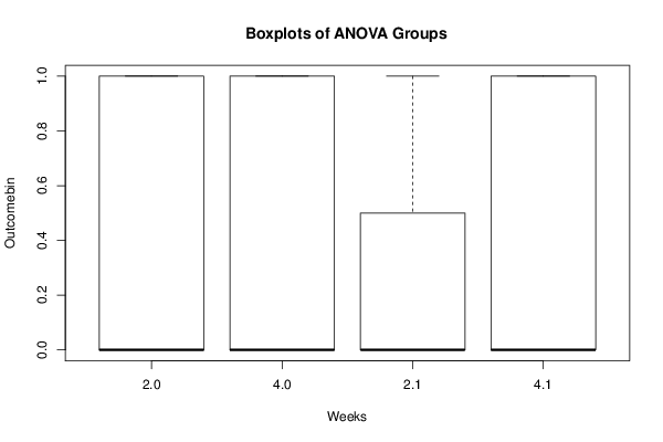
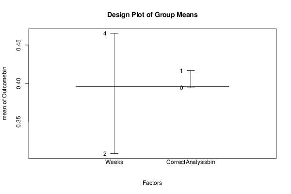
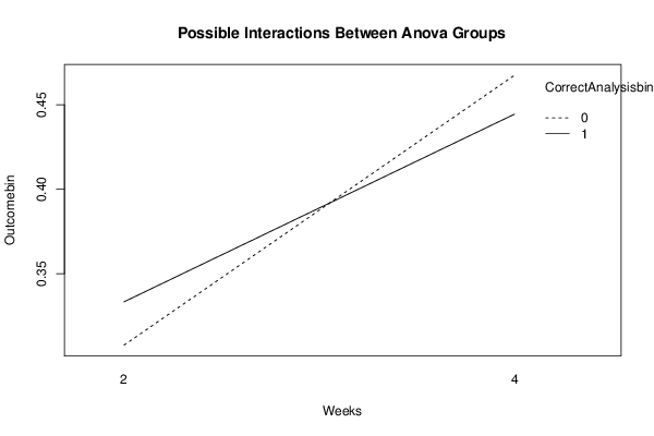
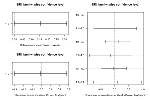
Figures (Output of Computation) | |||||||||||||||||||||||||||||||||||||||||||||||||||||||||||||||||||||||||||||||||||||||||||||||||||||||||||||||||||||||||||||||||||||||||||||||||||||||||||||||||||||||||||||||||||||||||||||||||||||||||||||||||||||||||||||||||||||||||||||||||||||||||||||||||||||||||||
Input Parameters & R Code | |||||||||||||||||||||||||||||||||||||||||||||||||||||||||||||||||||||||||||||||||||||||||||||||||||||||||||||||||||||||||||||||||||||||||||||||||||||||||||||||||||||||||||||||||||||||||||||||||||||||||||||||||||||||||||||||||||||||||||||||||||||||||||||||||||||||||||
| Parameters (Session): | |||||||||||||||||||||||||||||||||||||||||||||||||||||||||||||||||||||||||||||||||||||||||||||||||||||||||||||||||||||||||||||||||||||||||||||||||||||||||||||||||||||||||||||||||||||||||||||||||||||||||||||||||||||||||||||||||||||||||||||||||||||||||||||||||||||||||||
| par1 = 10 ; par2 = 1 ; par3 = 9 ; par4 = TRUE ; | |||||||||||||||||||||||||||||||||||||||||||||||||||||||||||||||||||||||||||||||||||||||||||||||||||||||||||||||||||||||||||||||||||||||||||||||||||||||||||||||||||||||||||||||||||||||||||||||||||||||||||||||||||||||||||||||||||||||||||||||||||||||||||||||||||||||||||
| Parameters (R input): | |||||||||||||||||||||||||||||||||||||||||||||||||||||||||||||||||||||||||||||||||||||||||||||||||||||||||||||||||||||||||||||||||||||||||||||||||||||||||||||||||||||||||||||||||||||||||||||||||||||||||||||||||||||||||||||||||||||||||||||||||||||||||||||||||||||||||||
| par1 = 10 ; par2 = 1 ; par3 = 9 ; par4 = TRUE ; | |||||||||||||||||||||||||||||||||||||||||||||||||||||||||||||||||||||||||||||||||||||||||||||||||||||||||||||||||||||||||||||||||||||||||||||||||||||||||||||||||||||||||||||||||||||||||||||||||||||||||||||||||||||||||||||||||||||||||||||||||||||||||||||||||||||||||||
| R code (references can be found in the software module): | |||||||||||||||||||||||||||||||||||||||||||||||||||||||||||||||||||||||||||||||||||||||||||||||||||||||||||||||||||||||||||||||||||||||||||||||||||||||||||||||||||||||||||||||||||||||||||||||||||||||||||||||||||||||||||||||||||||||||||||||||||||||||||||||||||||||||||
cat1 <- as.numeric(par1) # | |||||||||||||||||||||||||||||||||||||||||||||||||||||||||||||||||||||||||||||||||||||||||||||||||||||||||||||||||||||||||||||||||||||||||||||||||||||||||||||||||||||||||||||||||||||||||||||||||||||||||||||||||||||||||||||||||||||||||||||||||||||||||||||||||||||||||||