Free Statistics
of Irreproducible Research!
Description of Statistical Computation | |||||||||||||||||||||||||||||||||||||||||||||||||||||||||||||||||||||||||||||||||||||||||||||||||||||||||||||||||||||||||||||||||||||||||||||||||||||||||||||||||||||||||||||||||||||||||||||||||||||||||||||||||||||||||||||||||||||||||||||||||||||||||||||||||||||||||||||||||||||||||||||||||||||||||||||||||||||||||||||||||||||||||||||
|---|---|---|---|---|---|---|---|---|---|---|---|---|---|---|---|---|---|---|---|---|---|---|---|---|---|---|---|---|---|---|---|---|---|---|---|---|---|---|---|---|---|---|---|---|---|---|---|---|---|---|---|---|---|---|---|---|---|---|---|---|---|---|---|---|---|---|---|---|---|---|---|---|---|---|---|---|---|---|---|---|---|---|---|---|---|---|---|---|---|---|---|---|---|---|---|---|---|---|---|---|---|---|---|---|---|---|---|---|---|---|---|---|---|---|---|---|---|---|---|---|---|---|---|---|---|---|---|---|---|---|---|---|---|---|---|---|---|---|---|---|---|---|---|---|---|---|---|---|---|---|---|---|---|---|---|---|---|---|---|---|---|---|---|---|---|---|---|---|---|---|---|---|---|---|---|---|---|---|---|---|---|---|---|---|---|---|---|---|---|---|---|---|---|---|---|---|---|---|---|---|---|---|---|---|---|---|---|---|---|---|---|---|---|---|---|---|---|---|---|---|---|---|---|---|---|---|---|---|---|---|---|---|---|---|---|---|---|---|---|---|---|---|---|---|---|---|---|---|---|---|---|---|---|---|---|---|---|---|---|---|---|---|---|---|---|---|---|---|---|---|---|---|---|---|---|---|---|---|---|---|---|---|---|---|---|---|---|---|---|---|---|---|---|---|---|---|---|---|---|---|---|---|---|---|---|---|---|---|---|---|---|---|---|---|---|---|---|---|---|---|---|---|---|---|---|---|---|---|---|---|---|---|---|
| Author's title | |||||||||||||||||||||||||||||||||||||||||||||||||||||||||||||||||||||||||||||||||||||||||||||||||||||||||||||||||||||||||||||||||||||||||||||||||||||||||||||||||||||||||||||||||||||||||||||||||||||||||||||||||||||||||||||||||||||||||||||||||||||||||||||||||||||||||||||||||||||||||||||||||||||||||||||||||||||||||||||||||||||||||||||
| Author | *The author of this computation has been verified* | ||||||||||||||||||||||||||||||||||||||||||||||||||||||||||||||||||||||||||||||||||||||||||||||||||||||||||||||||||||||||||||||||||||||||||||||||||||||||||||||||||||||||||||||||||||||||||||||||||||||||||||||||||||||||||||||||||||||||||||||||||||||||||||||||||||||||||||||||||||||||||||||||||||||||||||||||||||||||||||||||||||||||||||
| R Software Module | rwasp_histogram.wasp | ||||||||||||||||||||||||||||||||||||||||||||||||||||||||||||||||||||||||||||||||||||||||||||||||||||||||||||||||||||||||||||||||||||||||||||||||||||||||||||||||||||||||||||||||||||||||||||||||||||||||||||||||||||||||||||||||||||||||||||||||||||||||||||||||||||||||||||||||||||||||||||||||||||||||||||||||||||||||||||||||||||||||||||
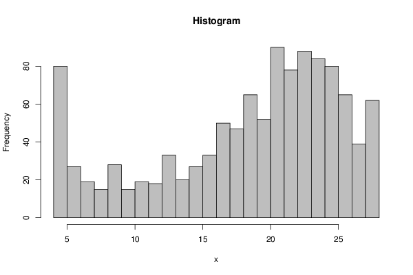
| Title produced by software | Histogram | ||||||||||||||||||||||||||||||||||||||||||||||||||||||||||||||||||||||||||||||||||||||||||||||||||||||||||||||||||||||||||||||||||||||||||||||||||||||||||||||||||||||||||||||||||||||||||||||||||||||||||||||||||||||||||||||||||||||||||||||||||||||||||||||||||||||||||||||||||||||||||||||||||||||||||||||||||||||||||||||||||||||||||||
| Date of computation | Fri, 21 Dec 2012 14:44:59 -0500 | ||||||||||||||||||||||||||||||||||||||||||||||||||||||||||||||||||||||||||||||||||||||||||||||||||||||||||||||||||||||||||||||||||||||||||||||||||||||||||||||||||||||||||||||||||||||||||||||||||||||||||||||||||||||||||||||||||||||||||||||||||||||||||||||||||||||||||||||||||||||||||||||||||||||||||||||||||||||||||||||||||||||||||||
| Cite this page as follows | Statistical Computations at FreeStatistics.org, Office for Research Development and Education, URL https://freestatistics.org/blog/index.php?v=date/2012/Dec/21/t13561191191fnf0355vniue2l.htm/, Retrieved Fri, 19 Apr 2024 23:56:42 +0000 | ||||||||||||||||||||||||||||||||||||||||||||||||||||||||||||||||||||||||||||||||||||||||||||||||||||||||||||||||||||||||||||||||||||||||||||||||||||||||||||||||||||||||||||||||||||||||||||||||||||||||||||||||||||||||||||||||||||||||||||||||||||||||||||||||||||||||||||||||||||||||||||||||||||||||||||||||||||||||||||||||||||||||||||
| Statistical Computations at FreeStatistics.org, Office for Research Development and Education, URL https://freestatistics.org/blog/index.php?pk=204165, Retrieved Fri, 19 Apr 2024 23:56:42 +0000 | |||||||||||||||||||||||||||||||||||||||||||||||||||||||||||||||||||||||||||||||||||||||||||||||||||||||||||||||||||||||||||||||||||||||||||||||||||||||||||||||||||||||||||||||||||||||||||||||||||||||||||||||||||||||||||||||||||||||||||||||||||||||||||||||||||||||||||||||||||||||||||||||||||||||||||||||||||||||||||||||||||||||||||||
| QR Codes: | |||||||||||||||||||||||||||||||||||||||||||||||||||||||||||||||||||||||||||||||||||||||||||||||||||||||||||||||||||||||||||||||||||||||||||||||||||||||||||||||||||||||||||||||||||||||||||||||||||||||||||||||||||||||||||||||||||||||||||||||||||||||||||||||||||||||||||||||||||||||||||||||||||||||||||||||||||||||||||||||||||||||||||||
|
| |||||||||||||||||||||||||||||||||||||||||||||||||||||||||||||||||||||||||||||||||||||||||||||||||||||||||||||||||||||||||||||||||||||||||||||||||||||||||||||||||||||||||||||||||||||||||||||||||||||||||||||||||||||||||||||||||||||||||||||||||||||||||||||||||||||||||||||||||||||||||||||||||||||||||||||||||||||||||||||||||||||||||||||
| Original text written by user: | |||||||||||||||||||||||||||||||||||||||||||||||||||||||||||||||||||||||||||||||||||||||||||||||||||||||||||||||||||||||||||||||||||||||||||||||||||||||||||||||||||||||||||||||||||||||||||||||||||||||||||||||||||||||||||||||||||||||||||||||||||||||||||||||||||||||||||||||||||||||||||||||||||||||||||||||||||||||||||||||||||||||||||||
| IsPrivate? | No (this computation is public) | ||||||||||||||||||||||||||||||||||||||||||||||||||||||||||||||||||||||||||||||||||||||||||||||||||||||||||||||||||||||||||||||||||||||||||||||||||||||||||||||||||||||||||||||||||||||||||||||||||||||||||||||||||||||||||||||||||||||||||||||||||||||||||||||||||||||||||||||||||||||||||||||||||||||||||||||||||||||||||||||||||||||||||||
| User-defined keywords | |||||||||||||||||||||||||||||||||||||||||||||||||||||||||||||||||||||||||||||||||||||||||||||||||||||||||||||||||||||||||||||||||||||||||||||||||||||||||||||||||||||||||||||||||||||||||||||||||||||||||||||||||||||||||||||||||||||||||||||||||||||||||||||||||||||||||||||||||||||||||||||||||||||||||||||||||||||||||||||||||||||||||||||
| Estimated Impact | 66 | ||||||||||||||||||||||||||||||||||||||||||||||||||||||||||||||||||||||||||||||||||||||||||||||||||||||||||||||||||||||||||||||||||||||||||||||||||||||||||||||||||||||||||||||||||||||||||||||||||||||||||||||||||||||||||||||||||||||||||||||||||||||||||||||||||||||||||||||||||||||||||||||||||||||||||||||||||||||||||||||||||||||||||||
Tree of Dependent Computations | |||||||||||||||||||||||||||||||||||||||||||||||||||||||||||||||||||||||||||||||||||||||||||||||||||||||||||||||||||||||||||||||||||||||||||||||||||||||||||||||||||||||||||||||||||||||||||||||||||||||||||||||||||||||||||||||||||||||||||||||||||||||||||||||||||||||||||||||||||||||||||||||||||||||||||||||||||||||||||||||||||||||||||||
| Family? (F = Feedback message, R = changed R code, M = changed R Module, P = changed Parameters, D = changed Data) | |||||||||||||||||||||||||||||||||||||||||||||||||||||||||||||||||||||||||||||||||||||||||||||||||||||||||||||||||||||||||||||||||||||||||||||||||||||||||||||||||||||||||||||||||||||||||||||||||||||||||||||||||||||||||||||||||||||||||||||||||||||||||||||||||||||||||||||||||||||||||||||||||||||||||||||||||||||||||||||||||||||||||||||
| - [Boxplot and Trimmed Means] [Reddy Moores Boxp...] [2010-10-12 16:37:57] [98fd0e87c3eb04e0cc2efde01dbafab6] - R P [Boxplot and Trimmed Means] [Reddy-Moores Plac...] [2010-10-13 09:46:26] [98fd0e87c3eb04e0cc2efde01dbafab6] - RMPD [Notched Boxplots] [] [2010-10-15 11:13:23] [b98453cac15ba1066b407e146608df68] - R D [Notched Boxplots] [Notched Boxplots ] [2012-12-11 13:08:43] [46762b18b00d15214a19b2ee3ead9dc9] - RMPD [Histogram] [histogram] [2012-12-21 19:28:34] [46762b18b00d15214a19b2ee3ead9dc9] - R [Histogram] [his] [2012-12-21 19:44:59] [9f1ef512d1eac2da3e1af89c6a547aff] [Current] - [Histogram] [histogram] [2012-12-21 19:55:34] [46762b18b00d15214a19b2ee3ead9dc9] - RM D [Stem-and-leaf Plot] [s a l] [2012-12-21 20:17:36] [46762b18b00d15214a19b2ee3ead9dc9] - RM D [Two-Way ANOVA] [anova 2 way] [2012-12-21 22:40:07] [46762b18b00d15214a19b2ee3ead9dc9] - RM D [Multiple Regression] [multiple] [2012-12-21 22:50:54] [46762b18b00d15214a19b2ee3ead9dc9] | |||||||||||||||||||||||||||||||||||||||||||||||||||||||||||||||||||||||||||||||||||||||||||||||||||||||||||||||||||||||||||||||||||||||||||||||||||||||||||||||||||||||||||||||||||||||||||||||||||||||||||||||||||||||||||||||||||||||||||||||||||||||||||||||||||||||||||||||||||||||||||||||||||||||||||||||||||||||||||||||||||||||||||||
| Feedback Forum | |||||||||||||||||||||||||||||||||||||||||||||||||||||||||||||||||||||||||||||||||||||||||||||||||||||||||||||||||||||||||||||||||||||||||||||||||||||||||||||||||||||||||||||||||||||||||||||||||||||||||||||||||||||||||||||||||||||||||||||||||||||||||||||||||||||||||||||||||||||||||||||||||||||||||||||||||||||||||||||||||||||||||||||
Post a new message | |||||||||||||||||||||||||||||||||||||||||||||||||||||||||||||||||||||||||||||||||||||||||||||||||||||||||||||||||||||||||||||||||||||||||||||||||||||||||||||||||||||||||||||||||||||||||||||||||||||||||||||||||||||||||||||||||||||||||||||||||||||||||||||||||||||||||||||||||||||||||||||||||||||||||||||||||||||||||||||||||||||||||||||
Dataset | |||||||||||||||||||||||||||||||||||||||||||||||||||||||||||||||||||||||||||||||||||||||||||||||||||||||||||||||||||||||||||||||||||||||||||||||||||||||||||||||||||||||||||||||||||||||||||||||||||||||||||||||||||||||||||||||||||||||||||||||||||||||||||||||||||||||||||||||||||||||||||||||||||||||||||||||||||||||||||||||||||||||||||||
| Dataseries X: | |||||||||||||||||||||||||||||||||||||||||||||||||||||||||||||||||||||||||||||||||||||||||||||||||||||||||||||||||||||||||||||||||||||||||||||||||||||||||||||||||||||||||||||||||||||||||||||||||||||||||||||||||||||||||||||||||||||||||||||||||||||||||||||||||||||||||||||||||||||||||||||||||||||||||||||||||||||||||||||||||||||||||||||
26 20 19 19 20 25 25 22 26 22 17 22 19 24 26 21 13 26 20 22 14 21 7 23 17 25 25 19 20 23 22 22 21 15 20 22 18 20 28 22 18 23 20 25 26 15 17 23 21 13 18 19 22 16 24 18 20 24 14 22 24 18 21 23 17 22 24 21 22 16 21 23 22 24 24 16 16 21 26 15 25 18 23 20 17 25 24 17 19 20 15 27 22 23 16 19 25 19 19 26 21 20 24 22 20 18 18 24 24 22 23 22 20 18 25 18 16 20 19 15 19 19 16 17 28 23 25 20 17 23 16 23 11 18 24 23 21 16 24 23 18 20 9 24 25 20 21 25 22 21 21 22 27 24 24 21 18 16 22 20 18 20 21 16 19 18 16 23 17 12 19 16 19 20 13 20 27 17 8 25 26 13 19 15 5 16 14 24 24 9 19 19 25 19 18 15 12 21 12 15 28 25 19 20 24 26 25 12 12 15 17 14 16 11 20 11 22 20 19 17 21 23 18 17 27 25 19 22 24 20 19 11 22 22 16 20 24 16 16 22 24 16 27 11 21 20 20 27 20 12 8 21 18 24 16 18 20 20 19 17 16 26 15 22 17 23 21 19 14 17 12 24 18 20 16 20 22 12 16 17 22 12 14 23 15 17 28 20 23 13 18 23 19 23 12 16 23 13 22 18 23 20 10 17 18 15 23 17 17 22 20 20 19 18 22 20 22 18 16 16 16 16 17 18 21 15 18 11 8 19 4 20 16 14 10 13 14 8 23 11 9 24 5 15 5 19 6 13 11 17 17 5 9 15 17 17 20 12 7 16 7 14 24 15 15 10 14 18 12 9 9 8 18 10 17 14 16 10 19 10 14 10 4 19 9 12 16 11 18 11 24 17 18 9 19 18 12 23 22 14 14 16 23 7 10 12 12 12 17 21 16 11 14 13 9 19 13 19 13 13 13 14 12 22 11 5 18 19 14 15 12 19 15 17 8 10 12 12 20 12 12 14 6 10 18 18 7 18 9 17 22 11 15 17 15 22 9 13 20 14 14 12 20 20 8 17 9 18 22 10 13 15 18 18 12 12 20 12 16 16 18 16 13 17 13 17 23 24 22 20 24 27 28 27 24 23 24 27 27 28 27 23 24 28 27 25 19 24 20 28 26 23 23 20 11 24 25 23 18 20 20 24 23 25 28 26 26 23 22 24 21 20 22 20 25 20 22 23 25 23 23 22 24 25 21 12 17 20 23 23 20 28 24 24 24 24 28 25 21 25 25 18 17 26 28 21 27 22 21 25 22 23 26 19 25 21 13 24 25 26 25 25 22 21 23 25 24 21 21 25 22 20 20 23 28 23 28 24 18 20 28 21 21 25 19 18 21 22 24 15 28 26 23 26 20 22 20 23 22 24 23 22 26 23 27 23 21 26 23 21 27 19 23 25 23 22 22 25 25 28 28 20 25 19 25 22 18 20 17 17 18 21 20 28 19 22 16 18 25 17 14 11 27 20 22 22 21 23 17 24 14 17 23 24 24 8 22 23 25 21 24 15 22 21 25 16 28 23 21 21 26 22 21 18 12 25 17 24 15 13 26 16 24 21 20 14 25 25 20 22 20 26 18 22 24 17 24 20 19 20 15 23 26 22 20 24 26 21 25 13 20 22 23 28 22 20 6 21 20 18 23 20 24 22 21 18 21 23 23 15 21 24 23 21 21 20 11 22 27 25 18 20 24 10 27 21 21 18 15 24 22 14 28 18 26 17 19 22 18 24 15 18 26 11 26 21 23 23 15 22 26 16 20 18 22 16 19 20 19 23 24 25 21 21 23 27 23 18 16 16 23 20 20 21 24 22 23 20 25 23 27 27 22 24 25 22 28 28 27 25 16 28 21 24 27 14 14 27 20 21 22 21 12 20 24 19 28 23 27 22 27 26 22 21 19 24 19 26 22 28 21 23 28 10 24 21 21 24 24 25 25 23 21 16 17 25 24 23 25 23 28 26 22 19 26 18 18 25 27 12 15 21 23 22 21 24 27 22 28 26 10 19 22 21 24 25 21 20 21 24 23 18 24 24 19 20 18 20 27 23 26 23 17 21 25 23 27 24 20 27 21 24 21 15 25 25 22 24 21 22 23 22 20 23 25 23 22 25 26 22 24 24 25 20 26 21 26 21 22 16 26 28 18 25 23 21 20 25 22 21 16 18 4 4 6 8 8 4 4 8 5 4 4 4 4 4 4 8 4 4 4 8 4 7 4 4 5 4 4 4 4 4 4 4 15 10 4 8 4 4 4 4 7 4 6 5 4 16 5 12 6 9 9 4 5 4 4 5 4 4 4 5 4 6 4 4 18 4 6 4 4 5 4 4 5 10 5 8 8 5 4 4 4 5 4 4 8 4 5 14 8 8 4 4 6 4 7 7 4 6 4 7 4 4 8 4 4 10 8 6 4 4 4 5 4 6 4 5 7 8 5 8 10 8 5 12 4 5 4 6 4 4 7 7 10 4 5 8 11 7 4 8 6 7 5 4 8 4 8 6 4 9 5 6 4 4 4 5 6 16 6 6 4 4 | |||||||||||||||||||||||||||||||||||||||||||||||||||||||||||||||||||||||||||||||||||||||||||||||||||||||||||||||||||||||||||||||||||||||||||||||||||||||||||||||||||||||||||||||||||||||||||||||||||||||||||||||||||||||||||||||||||||||||||||||||||||||||||||||||||||||||||||||||||||||||||||||||||||||||||||||||||||||||||||||||||||||||||||
Tables (Output of Computation) | |||||||||||||||||||||||||||||||||||||||||||||||||||||||||||||||||||||||||||||||||||||||||||||||||||||||||||||||||||||||||||||||||||||||||||||||||||||||||||||||||||||||||||||||||||||||||||||||||||||||||||||||||||||||||||||||||||||||||||||||||||||||||||||||||||||||||||||||||||||||||||||||||||||||||||||||||||||||||||||||||||||||||||||
| |||||||||||||||||||||||||||||||||||||||||||||||||||||||||||||||||||||||||||||||||||||||||||||||||||||||||||||||||||||||||||||||||||||||||||||||||||||||||||||||||||||||||||||||||||||||||||||||||||||||||||||||||||||||||||||||||||||||||||||||||||||||||||||||||||||||||||||||||||||||||||||||||||||||||||||||||||||||||||||||||||||||||||||
Figures (Output of Computation) | |||||||||||||||||||||||||||||||||||||||||||||||||||||||||||||||||||||||||||||||||||||||||||||||||||||||||||||||||||||||||||||||||||||||||||||||||||||||||||||||||||||||||||||||||||||||||||||||||||||||||||||||||||||||||||||||||||||||||||||||||||||||||||||||||||||||||||||||||||||||||||||||||||||||||||||||||||||||||||||||||||||||||||||
Input Parameters & R Code | |||||||||||||||||||||||||||||||||||||||||||||||||||||||||||||||||||||||||||||||||||||||||||||||||||||||||||||||||||||||||||||||||||||||||||||||||||||||||||||||||||||||||||||||||||||||||||||||||||||||||||||||||||||||||||||||||||||||||||||||||||||||||||||||||||||||||||||||||||||||||||||||||||||||||||||||||||||||||||||||||||||||||||||
| Parameters (Session): | |||||||||||||||||||||||||||||||||||||||||||||||||||||||||||||||||||||||||||||||||||||||||||||||||||||||||||||||||||||||||||||||||||||||||||||||||||||||||||||||||||||||||||||||||||||||||||||||||||||||||||||||||||||||||||||||||||||||||||||||||||||||||||||||||||||||||||||||||||||||||||||||||||||||||||||||||||||||||||||||||||||||||||||
| par1 = 162 ; par2 = grey ; par3 = FALSE ; par4 = Unknown ; | |||||||||||||||||||||||||||||||||||||||||||||||||||||||||||||||||||||||||||||||||||||||||||||||||||||||||||||||||||||||||||||||||||||||||||||||||||||||||||||||||||||||||||||||||||||||||||||||||||||||||||||||||||||||||||||||||||||||||||||||||||||||||||||||||||||||||||||||||||||||||||||||||||||||||||||||||||||||||||||||||||||||||||||
| Parameters (R input): | |||||||||||||||||||||||||||||||||||||||||||||||||||||||||||||||||||||||||||||||||||||||||||||||||||||||||||||||||||||||||||||||||||||||||||||||||||||||||||||||||||||||||||||||||||||||||||||||||||||||||||||||||||||||||||||||||||||||||||||||||||||||||||||||||||||||||||||||||||||||||||||||||||||||||||||||||||||||||||||||||||||||||||||
| par1 = 28 ; par2 = grey ; par3 = FALSE ; par4 = Unknown ; | |||||||||||||||||||||||||||||||||||||||||||||||||||||||||||||||||||||||||||||||||||||||||||||||||||||||||||||||||||||||||||||||||||||||||||||||||||||||||||||||||||||||||||||||||||||||||||||||||||||||||||||||||||||||||||||||||||||||||||||||||||||||||||||||||||||||||||||||||||||||||||||||||||||||||||||||||||||||||||||||||||||||||||||
| R code (references can be found in the software module): | |||||||||||||||||||||||||||||||||||||||||||||||||||||||||||||||||||||||||||||||||||||||||||||||||||||||||||||||||||||||||||||||||||||||||||||||||||||||||||||||||||||||||||||||||||||||||||||||||||||||||||||||||||||||||||||||||||||||||||||||||||||||||||||||||||||||||||||||||||||||||||||||||||||||||||||||||||||||||||||||||||||||||||||
par1 <- as.numeric(par1) | |||||||||||||||||||||||||||||||||||||||||||||||||||||||||||||||||||||||||||||||||||||||||||||||||||||||||||||||||||||||||||||||||||||||||||||||||||||||||||||||||||||||||||||||||||||||||||||||||||||||||||||||||||||||||||||||||||||||||||||||||||||||||||||||||||||||||||||||||||||||||||||||||||||||||||||||||||||||||||||||||||||||||||||