Free Statistics
of Irreproducible Research!
Description of Statistical Computation | |||||||||||||||||||||||||||||||||||||||||||||||||||||
|---|---|---|---|---|---|---|---|---|---|---|---|---|---|---|---|---|---|---|---|---|---|---|---|---|---|---|---|---|---|---|---|---|---|---|---|---|---|---|---|---|---|---|---|---|---|---|---|---|---|---|---|---|---|
| Author's title | |||||||||||||||||||||||||||||||||||||||||||||||||||||
| Author | *The author of this computation has been verified* | ||||||||||||||||||||||||||||||||||||||||||||||||||||
| R Software Module | -- | ||||||||||||||||||||||||||||||||||||||||||||||||||||
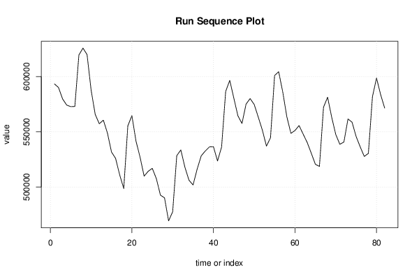
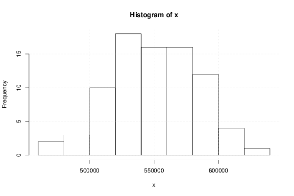
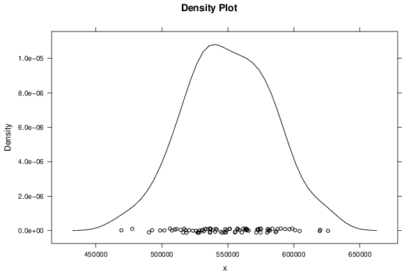
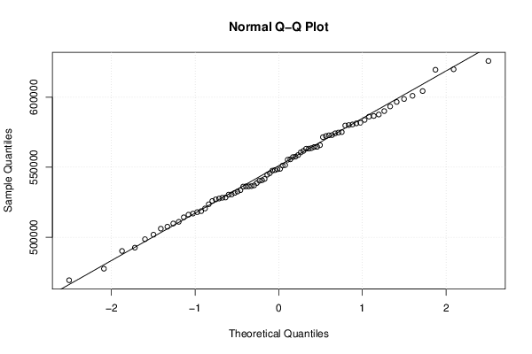
| Title produced by software | Univariate Explorative Data Analysis | ||||||||||||||||||||||||||||||||||||||||||||||||||||
| Date of computation | Thu, 20 Dec 2012 20:14:13 -0500 | ||||||||||||||||||||||||||||||||||||||||||||||||||||
| Cite this page as follows | Statistical Computations at FreeStatistics.org, Office for Research Development and Education, URL https://freestatistics.org/blog/index.php?v=date/2012/Dec/20/t1356052469lm50hsc1gel0swg.htm/, Retrieved Sun, 06 Jul 2025 02:27:14 +0000 | ||||||||||||||||||||||||||||||||||||||||||||||||||||
| Statistical Computations at FreeStatistics.org, Office for Research Development and Education, URL https://freestatistics.org/blog/index.php?pk=203236, Retrieved Sun, 06 Jul 2025 02:27:14 +0000 | |||||||||||||||||||||||||||||||||||||||||||||||||||||
| QR Codes: | |||||||||||||||||||||||||||||||||||||||||||||||||||||
|
| |||||||||||||||||||||||||||||||||||||||||||||||||||||
| Original text written by user: | |||||||||||||||||||||||||||||||||||||||||||||||||||||
| IsPrivate? | No (this computation is public) | ||||||||||||||||||||||||||||||||||||||||||||||||||||
| User-defined keywords | |||||||||||||||||||||||||||||||||||||||||||||||||||||
| Estimated Impact | 220 | ||||||||||||||||||||||||||||||||||||||||||||||||||||
Tree of Dependent Computations | |||||||||||||||||||||||||||||||||||||||||||||||||||||
| Family? (F = Feedback message, R = changed R code, M = changed R Module, P = changed Parameters, D = changed Data) | |||||||||||||||||||||||||||||||||||||||||||||||||||||
| - [Univariate Explorative Data Analysis] [time effect in su...] [2010-11-17 08:55:33] [b98453cac15ba1066b407e146608df68] - R D [Univariate Explorative Data Analysis] [Workshop 7 (1)] [2012-11-17 15:28:24] [e31fe164d58995c48777312ee804d655] - R [Univariate Explorative Data Analysis] [workshop 7 b] [2012-11-18 11:29:34] [dbae308bdff61c0f4902cc85498d0d35] - R D [Univariate Explorative Data Analysis] [Run sequence plot...] [2012-11-19 14:26:33] [8c30f4dd45e15fd207e4faf2fdf6253e] - M [Univariate Explorative Data Analysis] [] [2012-12-21 01:14:13] [ab4290de075ebbfc5b460761b0110080] [Current] | |||||||||||||||||||||||||||||||||||||||||||||||||||||
| Feedback Forum | |||||||||||||||||||||||||||||||||||||||||||||||||||||
Post a new message | |||||||||||||||||||||||||||||||||||||||||||||||||||||
Dataset | |||||||||||||||||||||||||||||||||||||||||||||||||||||
| Dataseries X: | |||||||||||||||||||||||||||||||||||||||||||||||||||||
593408 590072 579799 574205 572775 572942 619567 625809 619916 587625 565742 557274 560576 548854 531673 525919 511038 498662 555362 564591 541657 527070 509846 514258 516922 507561 492622 490243 469357 477580 528379 533590 517945 506174 501866 516141 528222 532638 536322 536535 523597 536214 586570 596594 580523 564478 557560 575093 580112 574761 563250 551531 537034 544686 600991 604378 586111 563668 548604 551174 555654 547970 540324 530577 520579 518654 572273 581302 563280 547612 538712 540735 561649 558685 545732 536352 527676 530455 581744 598714 583775 571477 | |||||||||||||||||||||||||||||||||||||||||||||||||||||
Tables (Output of Computation) | |||||||||||||||||||||||||||||||||||||||||||||||||||||
| |||||||||||||||||||||||||||||||||||||||||||||||||||||
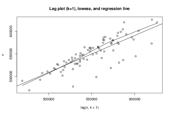
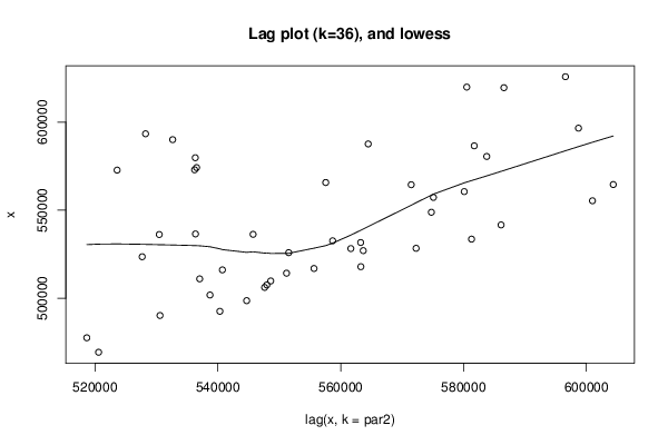
Figures (Output of Computation) | |||||||||||||||||||||||||||||||||||||||||||||||||||||
Input Parameters & R Code | |||||||||||||||||||||||||||||||||||||||||||||||||||||
| Parameters (Session): | |||||||||||||||||||||||||||||||||||||||||||||||||||||
| par1 = 0 ; par2 = 36 ; | |||||||||||||||||||||||||||||||||||||||||||||||||||||
| Parameters (R input): | |||||||||||||||||||||||||||||||||||||||||||||||||||||
| par1 = 0 ; par2 = 36 ; par3 = ; par4 = ; par5 = ; par6 = ; par7 = ; par8 = ; par9 = ; par10 = ; par11 = ; par12 = ; par13 = ; par14 = ; par15 = ; par16 = ; par17 = ; par18 = ; par19 = ; par20 = ; | |||||||||||||||||||||||||||||||||||||||||||||||||||||
| R code (references can be found in the software module): | |||||||||||||||||||||||||||||||||||||||||||||||||||||
par1 <- as.numeric(par1) | |||||||||||||||||||||||||||||||||||||||||||||||||||||