Free Statistics
of Irreproducible Research!
Description of Statistical Computation | |||||||||||||||||||||||||||||||||||||||||||||||||||||||||
|---|---|---|---|---|---|---|---|---|---|---|---|---|---|---|---|---|---|---|---|---|---|---|---|---|---|---|---|---|---|---|---|---|---|---|---|---|---|---|---|---|---|---|---|---|---|---|---|---|---|---|---|---|---|---|---|---|---|
| Author's title | |||||||||||||||||||||||||||||||||||||||||||||||||||||||||
| Author | *The author of this computation has been verified* | ||||||||||||||||||||||||||||||||||||||||||||||||||||||||
| R Software Module | rwasp_edauni.wasp | ||||||||||||||||||||||||||||||||||||||||||||||||||||||||
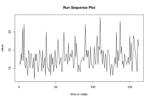
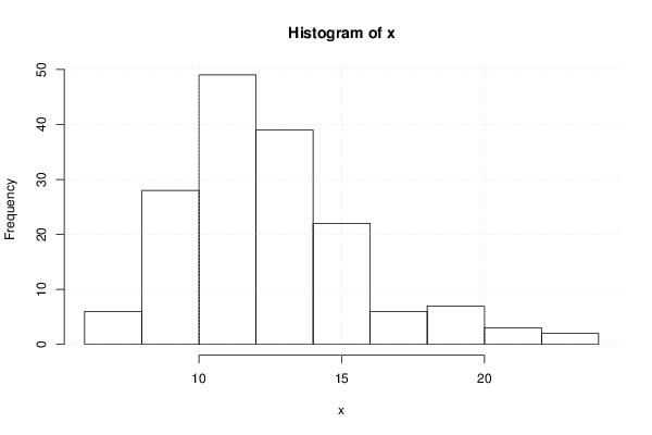
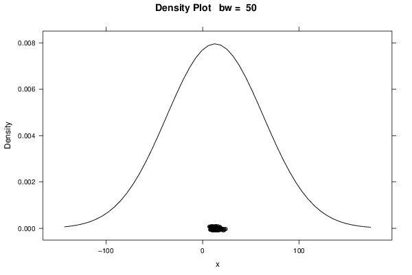
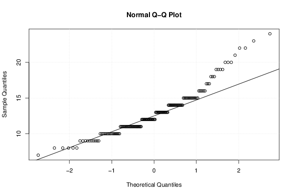
| Title produced by software | Univariate Explorative Data Analysis | ||||||||||||||||||||||||||||||||||||||||||||||||||||||||
| Date of computation | Thu, 20 Dec 2012 06:48:39 -0500 | ||||||||||||||||||||||||||||||||||||||||||||||||||||||||
| Cite this page as follows | Statistical Computations at FreeStatistics.org, Office for Research Development and Education, URL https://freestatistics.org/blog/index.php?v=date/2012/Dec/20/t13560041282g1l6il83r3cp3m.htm/, Retrieved Fri, 19 Apr 2024 01:19:58 +0000 | ||||||||||||||||||||||||||||||||||||||||||||||||||||||||
| Statistical Computations at FreeStatistics.org, Office for Research Development and Education, URL https://freestatistics.org/blog/index.php?pk=202632, Retrieved Fri, 19 Apr 2024 01:19:58 +0000 | |||||||||||||||||||||||||||||||||||||||||||||||||||||||||
| QR Codes: | |||||||||||||||||||||||||||||||||||||||||||||||||||||||||
|
| |||||||||||||||||||||||||||||||||||||||||||||||||||||||||
| Original text written by user: | |||||||||||||||||||||||||||||||||||||||||||||||||||||||||
| IsPrivate? | No (this computation is public) | ||||||||||||||||||||||||||||||||||||||||||||||||||||||||
| User-defined keywords | |||||||||||||||||||||||||||||||||||||||||||||||||||||||||
| Estimated Impact | 92 | ||||||||||||||||||||||||||||||||||||||||||||||||||||||||
Tree of Dependent Computations | |||||||||||||||||||||||||||||||||||||||||||||||||||||||||
| Family? (F = Feedback message, R = changed R code, M = changed R Module, P = changed Parameters, D = changed Data) | |||||||||||||||||||||||||||||||||||||||||||||||||||||||||
| - [Multiple Regression] [Competence to learn] [2010-11-17 07:43:53] [b98453cac15ba1066b407e146608df68] - PD [Multiple Regression] [] [2012-11-05 21:22:39] [43bd65bee76289cab2ce37423d405966] - RMPD [Univariate Explorative Data Analysis] [] [2012-12-20 11:48:39] [e8c322125b0cf2de4bdab96981906a22] [Current] - R [Univariate Explorative Data Analysis] [] [2012-12-22 22:17:32] [74be16979710d4c4e7c6647856088456] | |||||||||||||||||||||||||||||||||||||||||||||||||||||||||
| Feedback Forum | |||||||||||||||||||||||||||||||||||||||||||||||||||||||||
Post a new message | |||||||||||||||||||||||||||||||||||||||||||||||||||||||||
Dataset | |||||||||||||||||||||||||||||||||||||||||||||||||||||||||
| Dataseries X: | |||||||||||||||||||||||||||||||||||||||||||||||||||||||||
12 11 14 12 21 12 22 11 10 13 10 8 15 14 10 14 14 11 10 13 7 14 12 14 11 9 11 15 14 13 9 15 10 11 13 8 20 12 10 10 9 14 8 14 11 13 9 11 15 11 10 14 18 14 11 12 13 9 10 15 20 12 12 14 13 11 17 12 13 14 13 15 13 10 11 19 13 17 13 9 11 10 9 12 12 13 13 12 15 22 13 15 13 15 10 11 16 11 11 10 10 16 12 11 16 19 11 16 15 24 14 15 11 15 12 10 14 13 9 15 15 14 11 8 11 11 8 10 11 13 11 20 10 15 12 14 23 14 16 11 12 10 14 12 12 11 12 13 11 19 12 17 9 12 19 18 15 14 11 9 18 16 | |||||||||||||||||||||||||||||||||||||||||||||||||||||||||
Tables (Output of Computation) | |||||||||||||||||||||||||||||||||||||||||||||||||||||||||
| |||||||||||||||||||||||||||||||||||||||||||||||||||||||||
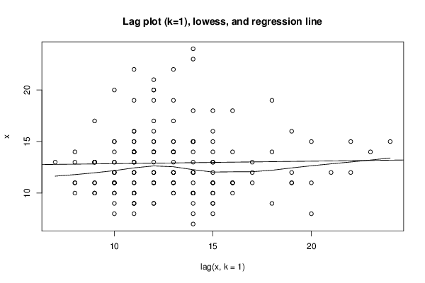
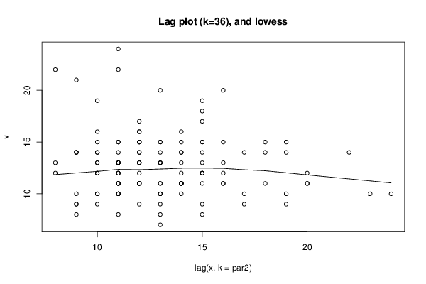
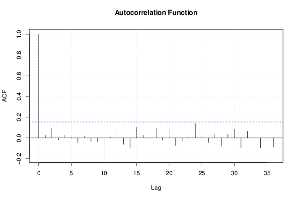
Figures (Output of Computation) | |||||||||||||||||||||||||||||||||||||||||||||||||||||||||
Input Parameters & R Code | |||||||||||||||||||||||||||||||||||||||||||||||||||||||||
| Parameters (Session): | |||||||||||||||||||||||||||||||||||||||||||||||||||||||||
| par1 = 50 ; par2 = 36 ; | |||||||||||||||||||||||||||||||||||||||||||||||||||||||||
| Parameters (R input): | |||||||||||||||||||||||||||||||||||||||||||||||||||||||||
| par1 = 50 ; par2 = 36 ; | |||||||||||||||||||||||||||||||||||||||||||||||||||||||||
| R code (references can be found in the software module): | |||||||||||||||||||||||||||||||||||||||||||||||||||||||||
par1 <- as.numeric(par1) | |||||||||||||||||||||||||||||||||||||||||||||||||||||||||