Repository of Reproducible Computations

Free Statistics

of Irreproducible Research!

Author's title

Author

*The author of this computation has been verified*

R Software Module

rwasp_autocorrelation.wasp

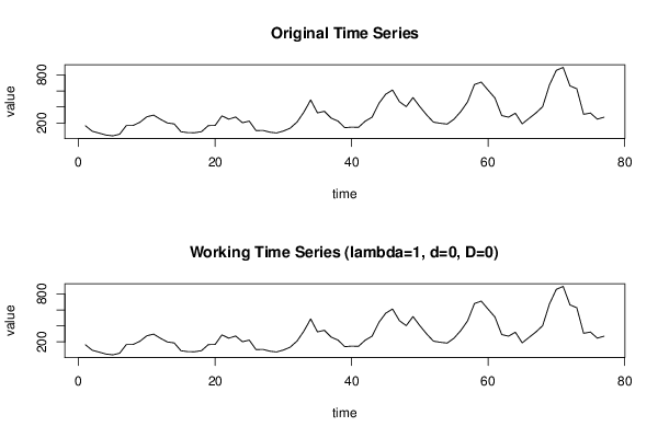
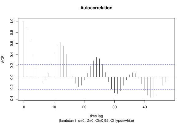
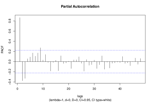
Title produced by software

(Partial) Autocorrelation Function

Date of computation

Mon, 17 Dec 2012 08:56:48 -0500

Cite this page as follows

Statistical Computations at FreeStatistics.org, Office for Research Development and Education, URL https://freestatistics.org/blog/index.php?v=date/2012/Dec/17/t1355752630tb517en2ykaaicy.htm/, Retrieved Thu, 18 Apr 2024 11:39:03 +0000

Statistical Computations at FreeStatistics.org, Office for Research Development and Education, URL https://freestatistics.org/blog/index.php?pk=200907, Retrieved Thu, 18 Apr 2024 11:39:03 +0000

QR Codes:

Paste this QR Code to cite your computation.

Original text written by user:

IsPrivate?

No (this computation is public)

User-defined keywords

Estimated Impact

185

Family? (F = Feedback message, R = changed R code, M = changed R Module, P = changed Parameters, D = changed Data)

-       [(Partial) Autocorrelation Function] [] [2012-12-17 13:56:48] [d76b387543b13b5e3afd8ff9e5fdc89f] [Current]
- RM      [(Partial) Autocorrelation Function] [] [2013-01-11 15:21:29] [74be16979710d4c4e7c6647856088456] 
- RM      [(Partial) Autocorrelation Function] [] [2013-01-11 15:21:29] [74be16979710d4c4e7c6647856088456] 
- RM      [(Partial) Autocorrelation Function] [] [2013-01-11 15:21:29] [74be16979710d4c4e7c6647856088456] 
- RMP     [Spectral Analysis] [] [2013-01-11 20:15:31] [391561951b5d7f721cfaa4f5575ab127] 
- RMP     [Spectral Analysis] [Examen_Aanvulling...] [2013-01-11 21:34:57] [391561951b5d7f721cfaa4f5575ab127] 

Feedback Forum

Post a new message

Dataseries X:

Download CSV

Histogram

Boxplots

Summary of computational transaction
Raw Input	view raw input (R code)
Raw Output	view raw output of R engine
Computing time	3 seconds
R Server	'Sir Ronald Aylmer Fisher' @ fisher.wessa.net

\begin{tabular}{lllllllll}
\hline
Summary of computational transaction \tabularnewline
Raw Input & view raw input (R code)  \tabularnewline
Raw Output & view raw output of R engine  \tabularnewline
Computing time & 3 seconds \tabularnewline
R Server & 'Sir Ronald Aylmer Fisher' @ fisher.wessa.net \tabularnewline
\hline
\end{tabular}
%Source: https://freestatistics.org/blog/index.php?pk=200907&T=0

[TABLE]
[ROW][C]Summary of computational transaction[/C][/ROW]
[ROW][C]Raw Input[/C][C]view raw input (R code) [/C][/ROW]
[ROW][C]Raw Output[/C][C]view raw output of R engine [/C][/ROW]
[ROW][C]Computing time[/C][C]3 seconds[/C][/ROW]
[ROW][C]R Server[/C][C]'Sir Ronald Aylmer Fisher' @ fisher.wessa.net[/C][/ROW]
[/TABLE]
Source: https://freestatistics.org/blog/index.php?pk=200907&T=0

Globally Unique Identifier (entire table): ba.freestatistics.org/blog/index.php?pk=200907&T=0

As an alternative you can also use a QR Code:

The GUIDs for individual cells are displayed in the table below:

Summary of computational transaction
Raw Input	view raw input (R code)
Raw Output	view raw output of R engine
Computing time	3 seconds
R Server	'Sir Ronald Aylmer Fisher' @ fisher.wessa.net

Autocorrelation Function
Time lag k	ACF(k)	T-STAT	P-value
1	0.866168	7.6006	0
2	0.656374	5.7597	0
3	0.385934	3.3866	0.000559
4	0.14865	1.3044	0.097992
5	-0.021896	-0.1921	0.424072
6	-0.083725	-0.7347	0.232381
7	-0.052388	-0.4597	0.323514
8	0.066224	0.5811	0.28143
9	0.250068	2.1943	0.015613
10	0.422818	3.7102	0.000195
11	0.566696	4.9727	2e-06
12	0.618873	5.4306	0
13	0.554915	4.8694	3e-06
14	0.406916	3.5707	0.000309
15	0.22274	1.9545	0.027134
16	0.018794	0.1649	0.434722
17	-0.113368	-0.9948	0.161476
18	-0.174979	-1.5354	0.064388
19	-0.14975	-1.3141	0.096365
20	-0.054376	-0.4771	0.317305
21	0.069926	0.6136	0.270645
22	0.193559	1.6985	0.046728
23	0.291334	2.5564	0.006271
24	0.352595	3.094	0.001376
25	0.327419	2.8731	0.002625
26	0.228836	2.008	0.024074
27	0.082039	0.7199	0.236885
28	-0.086293	-0.7572	0.225616
29	-0.216986	-1.904	0.03032
30	-0.286629	-2.5152	0.006991
31	-0.297029	-2.6064	0.00549
32	-0.249949	-2.1933	0.015652
33	-0.151165	-1.3265	0.094303
34	-0.051289	-0.4501	0.326966
35	0.039124	0.3433	0.366149
36	0.077623	0.6811	0.248913
37	0.061207	0.5371	0.296376
38	-0.021755	-0.1909	0.424554
39	-0.120975	-1.0616	0.145878
40	-0.245702	-2.156	0.017102
41	-0.327835	-2.8767	0.002598
42	-0.365361	-3.206	0.00098
43	-0.362453	-3.1805	0.00106
44	-0.313407	-2.7501	0.00371
45	-0.233788	-2.0515	0.02181
46	-0.149697	-1.3136	0.096444
47	-0.086059	-0.7552	0.226226
48	-0.040632	-0.3565	0.361204

\begin{tabular}{lllllllll}
\hline
Autocorrelation Function \tabularnewline
Time lag k & ACF(k) & T-STAT & P-value \tabularnewline
1 & 0.866168 & 7.6006 & 0 \tabularnewline
2 & 0.656374 & 5.7597 & 0 \tabularnewline
3 & 0.385934 & 3.3866 & 0.000559 \tabularnewline
4 & 0.14865 & 1.3044 & 0.097992 \tabularnewline
5 & -0.021896 & -0.1921 & 0.424072 \tabularnewline
6 & -0.083725 & -0.7347 & 0.232381 \tabularnewline
7 & -0.052388 & -0.4597 & 0.323514 \tabularnewline
8 & 0.066224 & 0.5811 & 0.28143 \tabularnewline
9 & 0.250068 & 2.1943 & 0.015613 \tabularnewline
10 & 0.422818 & 3.7102 & 0.000195 \tabularnewline
11 & 0.566696 & 4.9727 & 2e-06 \tabularnewline
12 & 0.618873 & 5.4306 & 0 \tabularnewline
13 & 0.554915 & 4.8694 & 3e-06 \tabularnewline
14 & 0.406916 & 3.5707 & 0.000309 \tabularnewline
15 & 0.22274 & 1.9545 & 0.027134 \tabularnewline
16 & 0.018794 & 0.1649 & 0.434722 \tabularnewline
17 & -0.113368 & -0.9948 & 0.161476 \tabularnewline
18 & -0.174979 & -1.5354 & 0.064388 \tabularnewline
19 & -0.14975 & -1.3141 & 0.096365 \tabularnewline
20 & -0.054376 & -0.4771 & 0.317305 \tabularnewline
21 & 0.069926 & 0.6136 & 0.270645 \tabularnewline
22 & 0.193559 & 1.6985 & 0.046728 \tabularnewline
23 & 0.291334 & 2.5564 & 0.006271 \tabularnewline
24 & 0.352595 & 3.094 & 0.001376 \tabularnewline
25 & 0.327419 & 2.8731 & 0.002625 \tabularnewline
26 & 0.228836 & 2.008 & 0.024074 \tabularnewline
27 & 0.082039 & 0.7199 & 0.236885 \tabularnewline
28 & -0.086293 & -0.7572 & 0.225616 \tabularnewline
29 & -0.216986 & -1.904 & 0.03032 \tabularnewline
30 & -0.286629 & -2.5152 & 0.006991 \tabularnewline
31 & -0.297029 & -2.6064 & 0.00549 \tabularnewline
32 & -0.249949 & -2.1933 & 0.015652 \tabularnewline
33 & -0.151165 & -1.3265 & 0.094303 \tabularnewline
34 & -0.051289 & -0.4501 & 0.326966 \tabularnewline
35 & 0.039124 & 0.3433 & 0.366149 \tabularnewline
36 & 0.077623 & 0.6811 & 0.248913 \tabularnewline
37 & 0.061207 & 0.5371 & 0.296376 \tabularnewline
38 & -0.021755 & -0.1909 & 0.424554 \tabularnewline
39 & -0.120975 & -1.0616 & 0.145878 \tabularnewline
40 & -0.245702 & -2.156 & 0.017102 \tabularnewline
41 & -0.327835 & -2.8767 & 0.002598 \tabularnewline
42 & -0.365361 & -3.206 & 0.00098 \tabularnewline
43 & -0.362453 & -3.1805 & 0.00106 \tabularnewline
44 & -0.313407 & -2.7501 & 0.00371 \tabularnewline
45 & -0.233788 & -2.0515 & 0.02181 \tabularnewline
46 & -0.149697 & -1.3136 & 0.096444 \tabularnewline
47 & -0.086059 & -0.7552 & 0.226226 \tabularnewline
48 & -0.040632 & -0.3565 & 0.361204 \tabularnewline
\hline
\end{tabular}
%Source: https://freestatistics.org/blog/index.php?pk=200907&T=1

[TABLE]
[ROW][C]Autocorrelation Function[/C][/ROW]
[ROW][C]Time lag k[/C][C]ACF(k)[/C][C]T-STAT[/C][C]P-value[/C][/ROW]
[ROW][C]1[/C][C]0.866168[/C][C]7.6006[/C][C]0[/C][/ROW]
[ROW][C]2[/C][C]0.656374[/C][C]5.7597[/C][C]0[/C][/ROW]
[ROW][C]3[/C][C]0.385934[/C][C]3.3866[/C][C]0.000559[/C][/ROW]
[ROW][C]4[/C][C]0.14865[/C][C]1.3044[/C][C]0.097992[/C][/ROW]
[ROW][C]5[/C][C]-0.021896[/C][C]-0.1921[/C][C]0.424072[/C][/ROW]
[ROW][C]6[/C][C]-0.083725[/C][C]-0.7347[/C][C]0.232381[/C][/ROW]
[ROW][C]7[/C][C]-0.052388[/C][C]-0.4597[/C][C]0.323514[/C][/ROW]
[ROW][C]8[/C][C]0.066224[/C][C]0.5811[/C][C]0.28143[/C][/ROW]
[ROW][C]9[/C][C]0.250068[/C][C]2.1943[/C][C]0.015613[/C][/ROW]
[ROW][C]10[/C][C]0.422818[/C][C]3.7102[/C][C]0.000195[/C][/ROW]
[ROW][C]11[/C][C]0.566696[/C][C]4.9727[/C][C]2e-06[/C][/ROW]
[ROW][C]12[/C][C]0.618873[/C][C]5.4306[/C][C]0[/C][/ROW]
[ROW][C]13[/C][C]0.554915[/C][C]4.8694[/C][C]3e-06[/C][/ROW]
[ROW][C]14[/C][C]0.406916[/C][C]3.5707[/C][C]0.000309[/C][/ROW]
[ROW][C]15[/C][C]0.22274[/C][C]1.9545[/C][C]0.027134[/C][/ROW]
[ROW][C]16[/C][C]0.018794[/C][C]0.1649[/C][C]0.434722[/C][/ROW]
[ROW][C]17[/C][C]-0.113368[/C][C]-0.9948[/C][C]0.161476[/C][/ROW]
[ROW][C]18[/C][C]-0.174979[/C][C]-1.5354[/C][C]0.064388[/C][/ROW]
[ROW][C]19[/C][C]-0.14975[/C][C]-1.3141[/C][C]0.096365[/C][/ROW]
[ROW][C]20[/C][C]-0.054376[/C][C]-0.4771[/C][C]0.317305[/C][/ROW]
[ROW][C]21[/C][C]0.069926[/C][C]0.6136[/C][C]0.270645[/C][/ROW]
[ROW][C]22[/C][C]0.193559[/C][C]1.6985[/C][C]0.046728[/C][/ROW]
[ROW][C]23[/C][C]0.291334[/C][C]2.5564[/C][C]0.006271[/C][/ROW]
[ROW][C]24[/C][C]0.352595[/C][C]3.094[/C][C]0.001376[/C][/ROW]
[ROW][C]25[/C][C]0.327419[/C][C]2.8731[/C][C]0.002625[/C][/ROW]
[ROW][C]26[/C][C]0.228836[/C][C]2.008[/C][C]0.024074[/C][/ROW]
[ROW][C]27[/C][C]0.082039[/C][C]0.7199[/C][C]0.236885[/C][/ROW]
[ROW][C]28[/C][C]-0.086293[/C][C]-0.7572[/C][C]0.225616[/C][/ROW]
[ROW][C]29[/C][C]-0.216986[/C][C]-1.904[/C][C]0.03032[/C][/ROW]
[ROW][C]30[/C][C]-0.286629[/C][C]-2.5152[/C][C]0.006991[/C][/ROW]
[ROW][C]31[/C][C]-0.297029[/C][C]-2.6064[/C][C]0.00549[/C][/ROW]
[ROW][C]32[/C][C]-0.249949[/C][C]-2.1933[/C][C]0.015652[/C][/ROW]
[ROW][C]33[/C][C]-0.151165[/C][C]-1.3265[/C][C]0.094303[/C][/ROW]
[ROW][C]34[/C][C]-0.051289[/C][C]-0.4501[/C][C]0.326966[/C][/ROW]
[ROW][C]35[/C][C]0.039124[/C][C]0.3433[/C][C]0.366149[/C][/ROW]
[ROW][C]36[/C][C]0.077623[/C][C]0.6811[/C][C]0.248913[/C][/ROW]
[ROW][C]37[/C][C]0.061207[/C][C]0.5371[/C][C]0.296376[/C][/ROW]
[ROW][C]38[/C][C]-0.021755[/C][C]-0.1909[/C][C]0.424554[/C][/ROW]
[ROW][C]39[/C][C]-0.120975[/C][C]-1.0616[/C][C]0.145878[/C][/ROW]
[ROW][C]40[/C][C]-0.245702[/C][C]-2.156[/C][C]0.017102[/C][/ROW]
[ROW][C]41[/C][C]-0.327835[/C][C]-2.8767[/C][C]0.002598[/C][/ROW]
[ROW][C]42[/C][C]-0.365361[/C][C]-3.206[/C][C]0.00098[/C][/ROW]
[ROW][C]43[/C][C]-0.362453[/C][C]-3.1805[/C][C]0.00106[/C][/ROW]
[ROW][C]44[/C][C]-0.313407[/C][C]-2.7501[/C][C]0.00371[/C][/ROW]
[ROW][C]45[/C][C]-0.233788[/C][C]-2.0515[/C][C]0.02181[/C][/ROW]
[ROW][C]46[/C][C]-0.149697[/C][C]-1.3136[/C][C]0.096444[/C][/ROW]
[ROW][C]47[/C][C]-0.086059[/C][C]-0.7552[/C][C]0.226226[/C][/ROW]
[ROW][C]48[/C][C]-0.040632[/C][C]-0.3565[/C][C]0.361204[/C][/ROW]
[/TABLE]
Source: https://freestatistics.org/blog/index.php?pk=200907&T=1

Globally Unique Identifier (entire table): ba.freestatistics.org/blog/index.php?pk=200907&T=1

As an alternative you can also use a QR Code:

The GUIDs for individual cells are displayed in the table below:

Autocorrelation Function
Time lag k	ACF(k)	T-STAT	P-value
1	0.866168	7.6006	0
2	0.656374	5.7597	0
3	0.385934	3.3866	0.000559
4	0.14865	1.3044	0.097992
5	-0.021896	-0.1921	0.424072
6	-0.083725	-0.7347	0.232381
7	-0.052388	-0.4597	0.323514
8	0.066224	0.5811	0.28143
9	0.250068	2.1943	0.015613
10	0.422818	3.7102	0.000195
11	0.566696	4.9727	2e-06
12	0.618873	5.4306	0
13	0.554915	4.8694	3e-06
14	0.406916	3.5707	0.000309
15	0.22274	1.9545	0.027134
16	0.018794	0.1649	0.434722
17	-0.113368	-0.9948	0.161476
18	-0.174979	-1.5354	0.064388
19	-0.14975	-1.3141	0.096365
20	-0.054376	-0.4771	0.317305
21	0.069926	0.6136	0.270645
22	0.193559	1.6985	0.046728
23	0.291334	2.5564	0.006271
24	0.352595	3.094	0.001376
25	0.327419	2.8731	0.002625
26	0.228836	2.008	0.024074
27	0.082039	0.7199	0.236885
28	-0.086293	-0.7572	0.225616
29	-0.216986	-1.904	0.03032
30	-0.286629	-2.5152	0.006991
31	-0.297029	-2.6064	0.00549
32	-0.249949	-2.1933	0.015652
33	-0.151165	-1.3265	0.094303
34	-0.051289	-0.4501	0.326966
35	0.039124	0.3433	0.366149
36	0.077623	0.6811	0.248913
37	0.061207	0.5371	0.296376
38	-0.021755	-0.1909	0.424554
39	-0.120975	-1.0616	0.145878
40	-0.245702	-2.156	0.017102
41	-0.327835	-2.8767	0.002598
42	-0.365361	-3.206	0.00098
43	-0.362453	-3.1805	0.00106
44	-0.313407	-2.7501	0.00371
45	-0.233788	-2.0515	0.02181
46	-0.149697	-1.3136	0.096444
47	-0.086059	-0.7552	0.226226
48	-0.040632	-0.3565	0.361204

Partial Autocorrelation Function
Time lag k	PACF(k)	T-STAT	P-value
1	0.866168	7.6006	0
2	-0.375865	-3.2982	0.000737
3	-0.329768	-2.8937	0.002475
4	0.057273	0.5026	0.30835
5	0.090923	0.7978	0.213707
6	0.170483	1.496	0.069373
7	0.107006	0.939	0.175341
8	0.170615	1.4971	0.069222
9	0.273232	2.3976	0.009463
10	0.032532	0.2855	0.388027
11	0.140535	1.2332	0.110628
12	-0.014899	-0.1307	0.44816
13	-0.185487	-1.6276	0.053844
14	-0.015012	-0.1317	0.447771
15	0.027318	0.2397	0.405593
16	-0.179636	-1.5763	0.059528
17	0.114863	1.0079	0.158324
18	-0.036633	-0.3215	0.374368
19	-0.025212	-0.2212	0.412747
20	0.008746	0.0767	0.469513
21	-0.136013	-1.1935	0.118167
22	0.035542	0.3119	0.377986
23	0.037471	0.3288	0.371596
24	0.095216	0.8355	0.203005
25	-0.032862	-0.2884	0.386922
26	-0.18703	-1.6412	0.052419
27	0.04138	0.3631	0.358758
28	-0.071064	-0.6236	0.267371
29	-0.058888	-0.5167	0.30341
30	0.030638	0.2688	0.394384
31	-0.135134	-1.1858	0.119674
32	-0.060775	-0.5333	0.297682
33	0.113499	0.996	0.161197
34	-0.149839	-1.3148	0.096235
35	-0.010882	-0.0955	0.462086
36	-0.125373	-1.1001	0.137349
37	-0.031224	-0.274	0.392413
38	-0.023364	-0.205	0.41905
39	-0.008987	-0.0789	0.468674
40	-0.01815	-0.1593	0.436937
41	0.100947	0.8858	0.18924
42	-0.035273	-0.3095	0.378883
43	-0.02448	-0.2148	0.415241
44	-0.079489	-0.6975	0.243792
45	0.002825	0.0248	0.490145
46	0.070309	0.617	0.269542
47	-0.052521	-0.4609	0.323095
48	0.061802	0.5423	0.294586

\begin{tabular}{lllllllll}
\hline
Partial Autocorrelation Function \tabularnewline
Time lag k & PACF(k) & T-STAT & P-value \tabularnewline
1 & 0.866168 & 7.6006 & 0 \tabularnewline
2 & -0.375865 & -3.2982 & 0.000737 \tabularnewline
3 & -0.329768 & -2.8937 & 0.002475 \tabularnewline
4 & 0.057273 & 0.5026 & 0.30835 \tabularnewline
5 & 0.090923 & 0.7978 & 0.213707 \tabularnewline
6 & 0.170483 & 1.496 & 0.069373 \tabularnewline
7 & 0.107006 & 0.939 & 0.175341 \tabularnewline
8 & 0.170615 & 1.4971 & 0.069222 \tabularnewline
9 & 0.273232 & 2.3976 & 0.009463 \tabularnewline
10 & 0.032532 & 0.2855 & 0.388027 \tabularnewline
11 & 0.140535 & 1.2332 & 0.110628 \tabularnewline
12 & -0.014899 & -0.1307 & 0.44816 \tabularnewline
13 & -0.185487 & -1.6276 & 0.053844 \tabularnewline
14 & -0.015012 & -0.1317 & 0.447771 \tabularnewline
15 & 0.027318 & 0.2397 & 0.405593 \tabularnewline
16 & -0.179636 & -1.5763 & 0.059528 \tabularnewline
17 & 0.114863 & 1.0079 & 0.158324 \tabularnewline
18 & -0.036633 & -0.3215 & 0.374368 \tabularnewline
19 & -0.025212 & -0.2212 & 0.412747 \tabularnewline
20 & 0.008746 & 0.0767 & 0.469513 \tabularnewline
21 & -0.136013 & -1.1935 & 0.118167 \tabularnewline
22 & 0.035542 & 0.3119 & 0.377986 \tabularnewline
23 & 0.037471 & 0.3288 & 0.371596 \tabularnewline
24 & 0.095216 & 0.8355 & 0.203005 \tabularnewline
25 & -0.032862 & -0.2884 & 0.386922 \tabularnewline
26 & -0.18703 & -1.6412 & 0.052419 \tabularnewline
27 & 0.04138 & 0.3631 & 0.358758 \tabularnewline
28 & -0.071064 & -0.6236 & 0.267371 \tabularnewline
29 & -0.058888 & -0.5167 & 0.30341 \tabularnewline
30 & 0.030638 & 0.2688 & 0.394384 \tabularnewline
31 & -0.135134 & -1.1858 & 0.119674 \tabularnewline
32 & -0.060775 & -0.5333 & 0.297682 \tabularnewline
33 & 0.113499 & 0.996 & 0.161197 \tabularnewline
34 & -0.149839 & -1.3148 & 0.096235 \tabularnewline
35 & -0.010882 & -0.0955 & 0.462086 \tabularnewline
36 & -0.125373 & -1.1001 & 0.137349 \tabularnewline
37 & -0.031224 & -0.274 & 0.392413 \tabularnewline
38 & -0.023364 & -0.205 & 0.41905 \tabularnewline
39 & -0.008987 & -0.0789 & 0.468674 \tabularnewline
40 & -0.01815 & -0.1593 & 0.436937 \tabularnewline
41 & 0.100947 & 0.8858 & 0.18924 \tabularnewline
42 & -0.035273 & -0.3095 & 0.378883 \tabularnewline
43 & -0.02448 & -0.2148 & 0.415241 \tabularnewline
44 & -0.079489 & -0.6975 & 0.243792 \tabularnewline
45 & 0.002825 & 0.0248 & 0.490145 \tabularnewline
46 & 0.070309 & 0.617 & 0.269542 \tabularnewline
47 & -0.052521 & -0.4609 & 0.323095 \tabularnewline
48 & 0.061802 & 0.5423 & 0.294586 \tabularnewline
\hline
\end{tabular}
%Source: https://freestatistics.org/blog/index.php?pk=200907&T=2

[TABLE]
[ROW][C]Partial Autocorrelation Function[/C][/ROW]
[ROW][C]Time lag k[/C][C]PACF(k)[/C][C]T-STAT[/C][C]P-value[/C][/ROW]
[ROW][C]1[/C][C]0.866168[/C][C]7.6006[/C][C]0[/C][/ROW]
[ROW][C]2[/C][C]-0.375865[/C][C]-3.2982[/C][C]0.000737[/C][/ROW]
[ROW][C]3[/C][C]-0.329768[/C][C]-2.8937[/C][C]0.002475[/C][/ROW]
[ROW][C]4[/C][C]0.057273[/C][C]0.5026[/C][C]0.30835[/C][/ROW]
[ROW][C]5[/C][C]0.090923[/C][C]0.7978[/C][C]0.213707[/C][/ROW]
[ROW][C]6[/C][C]0.170483[/C][C]1.496[/C][C]0.069373[/C][/ROW]
[ROW][C]7[/C][C]0.107006[/C][C]0.939[/C][C]0.175341[/C][/ROW]
[ROW][C]8[/C][C]0.170615[/C][C]1.4971[/C][C]0.069222[/C][/ROW]
[ROW][C]9[/C][C]0.273232[/C][C]2.3976[/C][C]0.009463[/C][/ROW]
[ROW][C]10[/C][C]0.032532[/C][C]0.2855[/C][C]0.388027[/C][/ROW]
[ROW][C]11[/C][C]0.140535[/C][C]1.2332[/C][C]0.110628[/C][/ROW]
[ROW][C]12[/C][C]-0.014899[/C][C]-0.1307[/C][C]0.44816[/C][/ROW]
[ROW][C]13[/C][C]-0.185487[/C][C]-1.6276[/C][C]0.053844[/C][/ROW]
[ROW][C]14[/C][C]-0.015012[/C][C]-0.1317[/C][C]0.447771[/C][/ROW]
[ROW][C]15[/C][C]0.027318[/C][C]0.2397[/C][C]0.405593[/C][/ROW]
[ROW][C]16[/C][C]-0.179636[/C][C]-1.5763[/C][C]0.059528[/C][/ROW]
[ROW][C]17[/C][C]0.114863[/C][C]1.0079[/C][C]0.158324[/C][/ROW]
[ROW][C]18[/C][C]-0.036633[/C][C]-0.3215[/C][C]0.374368[/C][/ROW]
[ROW][C]19[/C][C]-0.025212[/C][C]-0.2212[/C][C]0.412747[/C][/ROW]
[ROW][C]20[/C][C]0.008746[/C][C]0.0767[/C][C]0.469513[/C][/ROW]
[ROW][C]21[/C][C]-0.136013[/C][C]-1.1935[/C][C]0.118167[/C][/ROW]
[ROW][C]22[/C][C]0.035542[/C][C]0.3119[/C][C]0.377986[/C][/ROW]
[ROW][C]23[/C][C]0.037471[/C][C]0.3288[/C][C]0.371596[/C][/ROW]
[ROW][C]24[/C][C]0.095216[/C][C]0.8355[/C][C]0.203005[/C][/ROW]
[ROW][C]25[/C][C]-0.032862[/C][C]-0.2884[/C][C]0.386922[/C][/ROW]
[ROW][C]26[/C][C]-0.18703[/C][C]-1.6412[/C][C]0.052419[/C][/ROW]
[ROW][C]27[/C][C]0.04138[/C][C]0.3631[/C][C]0.358758[/C][/ROW]
[ROW][C]28[/C][C]-0.071064[/C][C]-0.6236[/C][C]0.267371[/C][/ROW]
[ROW][C]29[/C][C]-0.058888[/C][C]-0.5167[/C][C]0.30341[/C][/ROW]
[ROW][C]30[/C][C]0.030638[/C][C]0.2688[/C][C]0.394384[/C][/ROW]
[ROW][C]31[/C][C]-0.135134[/C][C]-1.1858[/C][C]0.119674[/C][/ROW]
[ROW][C]32[/C][C]-0.060775[/C][C]-0.5333[/C][C]0.297682[/C][/ROW]
[ROW][C]33[/C][C]0.113499[/C][C]0.996[/C][C]0.161197[/C][/ROW]
[ROW][C]34[/C][C]-0.149839[/C][C]-1.3148[/C][C]0.096235[/C][/ROW]
[ROW][C]35[/C][C]-0.010882[/C][C]-0.0955[/C][C]0.462086[/C][/ROW]
[ROW][C]36[/C][C]-0.125373[/C][C]-1.1001[/C][C]0.137349[/C][/ROW]
[ROW][C]37[/C][C]-0.031224[/C][C]-0.274[/C][C]0.392413[/C][/ROW]
[ROW][C]38[/C][C]-0.023364[/C][C]-0.205[/C][C]0.41905[/C][/ROW]
[ROW][C]39[/C][C]-0.008987[/C][C]-0.0789[/C][C]0.468674[/C][/ROW]
[ROW][C]40[/C][C]-0.01815[/C][C]-0.1593[/C][C]0.436937[/C][/ROW]
[ROW][C]41[/C][C]0.100947[/C][C]0.8858[/C][C]0.18924[/C][/ROW]
[ROW][C]42[/C][C]-0.035273[/C][C]-0.3095[/C][C]0.378883[/C][/ROW]
[ROW][C]43[/C][C]-0.02448[/C][C]-0.2148[/C][C]0.415241[/C][/ROW]
[ROW][C]44[/C][C]-0.079489[/C][C]-0.6975[/C][C]0.243792[/C][/ROW]
[ROW][C]45[/C][C]0.002825[/C][C]0.0248[/C][C]0.490145[/C][/ROW]
[ROW][C]46[/C][C]0.070309[/C][C]0.617[/C][C]0.269542[/C][/ROW]
[ROW][C]47[/C][C]-0.052521[/C][C]-0.4609[/C][C]0.323095[/C][/ROW]
[ROW][C]48[/C][C]0.061802[/C][C]0.5423[/C][C]0.294586[/C][/ROW]
[/TABLE]
Source: https://freestatistics.org/blog/index.php?pk=200907&T=2

Globally Unique Identifier (entire table): ba.freestatistics.org/blog/index.php?pk=200907&T=2

As an alternative you can also use a QR Code:

The GUIDs for individual cells are displayed in the table below:

Partial Autocorrelation Function
Time lag k	PACF(k)	T-STAT	P-value
1	0.866168	7.6006	0
2	-0.375865	-3.2982	0.000737
3	-0.329768	-2.8937	0.002475
4	0.057273	0.5026	0.30835
5	0.090923	0.7978	0.213707
6	0.170483	1.496	0.069373
7	0.107006	0.939	0.175341
8	0.170615	1.4971	0.069222
9	0.273232	2.3976	0.009463
10	0.032532	0.2855	0.388027
11	0.140535	1.2332	0.110628
12	-0.014899	-0.1307	0.44816
13	-0.185487	-1.6276	0.053844
14	-0.015012	-0.1317	0.447771
15	0.027318	0.2397	0.405593
16	-0.179636	-1.5763	0.059528
17	0.114863	1.0079	0.158324
18	-0.036633	-0.3215	0.374368
19	-0.025212	-0.2212	0.412747
20	0.008746	0.0767	0.469513
21	-0.136013	-1.1935	0.118167
22	0.035542	0.3119	0.377986
23	0.037471	0.3288	0.371596
24	0.095216	0.8355	0.203005
25	-0.032862	-0.2884	0.386922
26	-0.18703	-1.6412	0.052419
27	0.04138	0.3631	0.358758
28	-0.071064	-0.6236	0.267371
29	-0.058888	-0.5167	0.30341
30	0.030638	0.2688	0.394384
31	-0.135134	-1.1858	0.119674
32	-0.060775	-0.5333	0.297682
33	0.113499	0.996	0.161197
34	-0.149839	-1.3148	0.096235
35	-0.010882	-0.0955	0.462086
36	-0.125373	-1.1001	0.137349
37	-0.031224	-0.274	0.392413
38	-0.023364	-0.205	0.41905
39	-0.008987	-0.0789	0.468674
40	-0.01815	-0.1593	0.436937
41	0.100947	0.8858	0.18924
42	-0.035273	-0.3095	0.378883
43	-0.02448	-0.2148	0.415241
44	-0.079489	-0.6975	0.243792
45	0.002825	0.0248	0.490145
46	0.070309	0.617	0.269542
47	-0.052521	-0.4609	0.323095
48	0.061802	0.5423	0.294586

Figure 1

PNG link

Postscript link

PDF link

Figure 2

PNG link

Postscript link

PDF link

Figure 3

PNG link

Postscript link

PDF link

Parameters (Session):

par1 = 48 ; par2 = 1 ; par3 = 0 ; par4 = 0 ; par5 = 12 ; par6 = White Noise ; par7 = 0.95 ;

Parameters (R input):

par1 = 48 ; par2 = 1 ; par3 = 0 ; par4 = 0 ; par5 = 12 ; par6 = White Noise ; par7 = 0.95 ; par8 = ;

R code (references can be found in the software module):

if (par1 == 'Default') {
par1 = 10*log10(length(x))
} else {
par1 <- as.numeric(par1)
}
par2 <- as.numeric(par2)
par3 <- as.numeric(par3)
par4 <- as.numeric(par4)
par5 <- as.numeric(par5)
if (par6 == 'White Noise') par6 <- 'white' else par6 <- 'ma'
par7 <- as.numeric(par7)
if (par8 != '') par8 <- as.numeric(par8)
ox <- x
if (par8 == '') {
if (par2 == 0) {
x <- log(x)
} else {
x <- (x ^ par2 - 1) / par2
}
} else {
x <- log(x,base=par8)
}
if (par3 > 0) x <- diff(x,lag=1,difference=par3)
if (par4 > 0) x <- diff(x,lag=par5,difference=par4)
bitmap(file='picts.png')
op <- par(mfrow=c(2,1))
plot(ox,type='l',main='Original Time Series',xlab='time',ylab='value')
if (par8=='') {
mytitle <- paste('Working Time Series (lambda=',par2,', d=',par3,', D=',par4,')',sep='')
mysub <- paste('(lambda=',par2,', d=',par3,', D=',par4,', CI=', par7, ', CI type=',par6,')',sep='')
} else {
mytitle <- paste('Working Time Series (base=',par8,', d=',par3,', D=',par4,')',sep='')
mysub <- paste('(base=',par8,', d=',par3,', D=',par4,', CI=', par7, ', CI type=',par6,')',sep='')
}
plot(x,type='l', main=mytitle,xlab='time',ylab='value')
par(op)
dev.off()
bitmap(file='pic1.png')
racf <- acf(x, par1, main='Autocorrelation', xlab='time lag', ylab='ACF', ci.type=par6, ci=par7, sub=mysub)
dev.off()
bitmap(file='pic2.png')
rpacf <- pacf(x,par1,main='Partial Autocorrelation',xlab='lags',ylab='PACF',sub=mysub)
dev.off()
(myacf <- c(racf$acf))
(mypacf <- c(rpacf$acf))
lengthx <- length(x)
sqrtn <- sqrt(lengthx)
load(file='createtable')
a<-table.start()
a<-table.row.start(a)
a<-table.element(a,'Autocorrelation Function',4,TRUE)
a<-table.row.end(a)
a<-table.row.start(a)
a<-table.element(a,'Time lag k',header=TRUE)
a<-table.element(a,hyperlink('basics.htm','ACF(k)','click here for more information about the Autocorrelation Function'),header=TRUE)
a<-table.element(a,'T-STAT',header=TRUE)
a<-table.element(a,'P-value',header=TRUE)
a<-table.row.end(a)
for (i in 2:(par1+1)) {
a<-table.row.start(a)
a<-table.element(a,i-1,header=TRUE)
a<-table.element(a,round(myacf[i],6))
mytstat <- myacf[i]*sqrtn
a<-table.element(a,round(mytstat,4))
a<-table.element(a,round(1-pt(abs(mytstat),lengthx),6))
a<-table.row.end(a)
}
a<-table.end(a)
table.save(a,file='mytable.tab')
a<-table.start()
a<-table.row.start(a)
a<-table.element(a,'Partial Autocorrelation Function',4,TRUE)
a<-table.row.end(a)
a<-table.row.start(a)
a<-table.element(a,'Time lag k',header=TRUE)
a<-table.element(a,hyperlink('basics.htm','PACF(k)','click here for more information about the Partial Autocorrelation Function'),header=TRUE)
a<-table.element(a,'T-STAT',header=TRUE)
a<-table.element(a,'P-value',header=TRUE)
a<-table.row.end(a)
for (i in 1:par1) {
a<-table.row.start(a)
a<-table.element(a,i,header=TRUE)
a<-table.element(a,round(mypacf[i],6))
mytstat <- mypacf[i]*sqrtn
a<-table.element(a,round(mytstat,4))
a<-table.element(a,round(1-pt(abs(mytstat),lengthx),6))
a<-table.row.end(a)
}
a<-table.end(a)
table.save(a,file='mytable1.tab')

Free Statistics

Description of Statistical Computation

Tree of Dependent Computations

Dataset

Tables (Output of Computation)

Figures (Output of Computation)

Input Parameters & R Code