Repository of Reproducible Computations

Free Statistics

of Irreproducible Research!

Author's title

Author

*The author of this computation has been verified*

R Software Module

rwasp_arimaforecasting.wasp

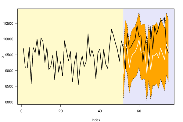
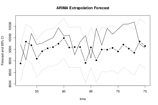
Title produced by software

ARIMA Forecasting

Date of computation

Sun, 16 Dec 2012 07:02:00 -0500

Cite this page as follows

Statistical Computations at FreeStatistics.org, Office for Research Development and Education, URL https://freestatistics.org/blog/index.php?v=date/2012/Dec/16/t1355659367aso77t44v1kjqy3.htm/, Retrieved Sat, 20 Apr 2024 10:33:30 +0000

Statistical Computations at FreeStatistics.org, Office for Research Development and Education, URL https://freestatistics.org/blog/index.php?pk=200265, Retrieved Sat, 20 Apr 2024 10:33:30 +0000

QR Codes:

Paste this QR Code to cite your computation.

Original text written by user:

IsPrivate?

No (this computation is public)

User-defined keywords

Estimated Impact

126

Family? (F = Feedback message, R = changed R code, M = changed R Module, P = changed Parameters, D = changed Data)

-     [Univariate Data Series] [web server] [2010-10-19 15:51:23] [b98453cac15ba1066b407e146608df68]
- RMP   [Variance Reduction Matrix] [Pageviews] [2010-11-29 10:12:20] [b98453cac15ba1066b407e146608df68]
- RM      [Standard Deviation-Mean Plot] [Pageviews] [2010-11-29 11:10:57] [b98453cac15ba1066b407e146608df68]
- RMP       [ARIMA Forecasting] [Pageviews] [2010-11-29 21:25:44] [b98453cac15ba1066b407e146608df68]
-   P         [ARIMA Forecasting] [Voorspelling met ...] [2012-11-29 15:52:07] [74be16979710d4c4e7c6647856088456]
-    D          [ARIMA Forecasting] [Voorspelling met ...] [2012-11-29 15:59:18] [74be16979710d4c4e7c6647856088456]
-   PD              [ARIMA Forecasting] [Voorspelling met ...] [2012-12-16 12:02:00] [c7a1fe63ca93df8f57ff0838e0a1dc12] [Current]

Feedback Forum

Post a new message

Dataseries X:

Download CSV

Histogram

Boxplots

Summary of computational transaction
Raw Input	view raw input (R code)
Raw Output	view raw output of R engine
Computing time	10 seconds
R Server	'Sir Maurice George Kendall' @ kendall.wessa.net

\begin{tabular}{lllllllll}
\hline
Summary of computational transaction \tabularnewline
Raw Input & view raw input (R code)  \tabularnewline
Raw Output & view raw output of R engine  \tabularnewline
Computing time & 10 seconds \tabularnewline
R Server & 'Sir Maurice George Kendall' @ kendall.wessa.net \tabularnewline
\hline
\end{tabular}
%Source: https://freestatistics.org/blog/index.php?pk=200265&T=0

[TABLE]
[ROW][C]Summary of computational transaction[/C][/ROW]
[ROW][C]Raw Input[/C][C]view raw input (R code) [/C][/ROW]
[ROW][C]Raw Output[/C][C]view raw output of R engine [/C][/ROW]
[ROW][C]Computing time[/C][C]10 seconds[/C][/ROW]
[ROW][C]R Server[/C][C]'Sir Maurice George Kendall' @ kendall.wessa.net[/C][/ROW]
[/TABLE]
Source: https://freestatistics.org/blog/index.php?pk=200265&T=0

Globally Unique Identifier (entire table): ba.freestatistics.org/blog/index.php?pk=200265&T=0

As an alternative you can also use a QR Code:

The GUIDs for individual cells are displayed in the table below:

Summary of computational transaction
Raw Input	view raw input (R code)
Raw Output	view raw output of R engine
Computing time	10 seconds
R Server	'Sir Maurice George Kendall' @ kendall.wessa.net

Univariate ARIMA Extrapolation Forecast
time	Y[t]	F[t]	95% LB	95% UB	p-value(H0: Y[t] = F[t])	P(F[t]>Y[t-1])	P(F[t]>Y[t-s])	P(F[t]>Y[51])
44	9069	-	-	-	-	-	-	-
45	9788	-	-	-	-	-	-	-
46	10312	-	-	-	-	-	-	-
47	10105	-	-	-	-	-	-	-
48	9863	-	-	-	-	-	-	-
49	9656	-	-	-	-	-	-	-
50	9295	-	-	-	-	-	-	-
51	9946	-	-	-	-	-	-	-
52	9701	8888.7374	8132.0503	9645.4245	0.0177	0.0031	0.0099	0.0031
53	9049	9828.3305	9069.8321	10586.829	0.022	0.6289	0.1057	0.3805
54	10190	9674.4212	8915.8475	10432.995	0.0914	0.9469	0.133	0.2414
55	9706	9093.2243	8291.1526	9895.296	0.0671	0.0037	0.03	0.0186
56	9765	9411.9711	8603.4903	10220.4519	0.196	0.238	0.2771	0.0977
57	9893	9541.6153	8733.6836	10349.547	0.197	0.2939	0.7252	0.1633
58	9994	9595.0483	8783.7544	10406.3423	0.1676	0.2358	0.1983	0.1983
59	10433	9741.4097	8874.9377	10607.8816	0.0589	0.2839	0.5364	0.3218
60	10073	9983.8416	9117.5702	10850.1129	0.4201	0.1548	0.9828	0.5341
61	10112	9578.8597	8712.0278	10445.6916	0.114	0.1319	0.0835	0.2032
62	9266	9596.4773	8723.8784	10469.0763	0.229	0.1234	0.4028	0.2162
63	9820	9596.1454	8721.6534	10470.6374	0.3079	0.7703	0.3525	0.2165
64	10097	8910.8372	8036.6502	9785.0242	0.0039	0.0208	0.0138	0.0101
65	9115	9579.9214	8705.4504	10454.3924	0.1487	0.1232	0.1767	0.206
66	10411	9027.7465	8066.564	9988.9291	0.0024	0.4294	0.0021	0.0306
67	9678	9487.8544	8526.222	10449.4868	0.3492	0.0299	0.1165	0.1752
68	10408	9482.656	8521.0517	10444.2603	0.0296	0.3453	0.0998	0.1725
69	10153	9559.1158	8588.167	10530.0647	0.1153	0.0433	0.723	0.2174
70	10368	9406.2833	8433.8477	10378.7188	0.0263	0.0662	0.2022	0.1383
71	10581	9704.3221	8733.1045	10675.5397	0.0384	0.0902	0.214	0.3129
72	10597	9530.383	8558.5126	10502.2533	0.0157	0.0171	0.7989	0.201
73	10680	9353.2809	8369.5091	10337.0527	0.0041	0.0066	0.0175	0.1188
74	9738	9839.297	8855.5877	10823.0062	0.42	0.047	0.626	0.4158
75	9556	9642.0824	8658.3185	10625.8463	0.4319	0.4242	0.0635	0.2724

\begin{tabular}{lllllllll}
\hline
Univariate ARIMA Extrapolation Forecast \tabularnewline
time & Y[t] & F[t] & 95% LB & 95% UB & p-value(H0: Y[t] = F[t]) & P(F[t]>Y[t-1]) & P(F[t]>Y[t-s]) & P(F[t]>Y[51]) \tabularnewline
44 & 9069 & - & - & - & - & - & - & - \tabularnewline
45 & 9788 & - & - & - & - & - & - & - \tabularnewline
46 & 10312 & - & - & - & - & - & - & - \tabularnewline
47 & 10105 & - & - & - & - & - & - & - \tabularnewline
48 & 9863 & - & - & - & - & - & - & - \tabularnewline
49 & 9656 & - & - & - & - & - & - & - \tabularnewline
50 & 9295 & - & - & - & - & - & - & - \tabularnewline
51 & 9946 & - & - & - & - & - & - & - \tabularnewline
52 & 9701 & 8888.7374 & 8132.0503 & 9645.4245 & 0.0177 & 0.0031 & 0.0099 & 0.0031 \tabularnewline
53 & 9049 & 9828.3305 & 9069.8321 & 10586.829 & 0.022 & 0.6289 & 0.1057 & 0.3805 \tabularnewline
54 & 10190 & 9674.4212 & 8915.8475 & 10432.995 & 0.0914 & 0.9469 & 0.133 & 0.2414 \tabularnewline
55 & 9706 & 9093.2243 & 8291.1526 & 9895.296 & 0.0671 & 0.0037 & 0.03 & 0.0186 \tabularnewline
56 & 9765 & 9411.9711 & 8603.4903 & 10220.4519 & 0.196 & 0.238 & 0.2771 & 0.0977 \tabularnewline
57 & 9893 & 9541.6153 & 8733.6836 & 10349.547 & 0.197 & 0.2939 & 0.7252 & 0.1633 \tabularnewline
58 & 9994 & 9595.0483 & 8783.7544 & 10406.3423 & 0.1676 & 0.2358 & 0.1983 & 0.1983 \tabularnewline
59 & 10433 & 9741.4097 & 8874.9377 & 10607.8816 & 0.0589 & 0.2839 & 0.5364 & 0.3218 \tabularnewline
60 & 10073 & 9983.8416 & 9117.5702 & 10850.1129 & 0.4201 & 0.1548 & 0.9828 & 0.5341 \tabularnewline
61 & 10112 & 9578.8597 & 8712.0278 & 10445.6916 & 0.114 & 0.1319 & 0.0835 & 0.2032 \tabularnewline
62 & 9266 & 9596.4773 & 8723.8784 & 10469.0763 & 0.229 & 0.1234 & 0.4028 & 0.2162 \tabularnewline
63 & 9820 & 9596.1454 & 8721.6534 & 10470.6374 & 0.3079 & 0.7703 & 0.3525 & 0.2165 \tabularnewline
64 & 10097 & 8910.8372 & 8036.6502 & 9785.0242 & 0.0039 & 0.0208 & 0.0138 & 0.0101 \tabularnewline
65 & 9115 & 9579.9214 & 8705.4504 & 10454.3924 & 0.1487 & 0.1232 & 0.1767 & 0.206 \tabularnewline
66 & 10411 & 9027.7465 & 8066.564 & 9988.9291 & 0.0024 & 0.4294 & 0.0021 & 0.0306 \tabularnewline
67 & 9678 & 9487.8544 & 8526.222 & 10449.4868 & 0.3492 & 0.0299 & 0.1165 & 0.1752 \tabularnewline
68 & 10408 & 9482.656 & 8521.0517 & 10444.2603 & 0.0296 & 0.3453 & 0.0998 & 0.1725 \tabularnewline
69 & 10153 & 9559.1158 & 8588.167 & 10530.0647 & 0.1153 & 0.0433 & 0.723 & 0.2174 \tabularnewline
70 & 10368 & 9406.2833 & 8433.8477 & 10378.7188 & 0.0263 & 0.0662 & 0.2022 & 0.1383 \tabularnewline
71 & 10581 & 9704.3221 & 8733.1045 & 10675.5397 & 0.0384 & 0.0902 & 0.214 & 0.3129 \tabularnewline
72 & 10597 & 9530.383 & 8558.5126 & 10502.2533 & 0.0157 & 0.0171 & 0.7989 & 0.201 \tabularnewline
73 & 10680 & 9353.2809 & 8369.5091 & 10337.0527 & 0.0041 & 0.0066 & 0.0175 & 0.1188 \tabularnewline
74 & 9738 & 9839.297 & 8855.5877 & 10823.0062 & 0.42 & 0.047 & 0.626 & 0.4158 \tabularnewline
75 & 9556 & 9642.0824 & 8658.3185 & 10625.8463 & 0.4319 & 0.4242 & 0.0635 & 0.2724 \tabularnewline
\hline
\end{tabular}
%Source: https://freestatistics.org/blog/index.php?pk=200265&T=1

[TABLE]
[ROW][C]Univariate ARIMA Extrapolation Forecast[/C][/ROW]
[ROW][C]time[/C][C]Y[t][/C][C]F[t][/C][C]95% LB[/C][C]95% UB[/C][C]p-value(H0: Y[t] = F[t])[/C][C]P(F[t]>Y[t-1])[/C][C]P(F[t]>Y[t-s])[/C][C]P(F[t]>Y[51])[/C][/ROW]
[ROW][C]44[/C][C]9069[/C][C]-[/C][C]-[/C][C]-[/C][C]-[/C][C]-[/C][C]-[/C][C]-[/C][/ROW]
[ROW][C]45[/C][C]9788[/C][C]-[/C][C]-[/C][C]-[/C][C]-[/C][C]-[/C][C]-[/C][C]-[/C][/ROW]
[ROW][C]46[/C][C]10312[/C][C]-[/C][C]-[/C][C]-[/C][C]-[/C][C]-[/C][C]-[/C][C]-[/C][/ROW]
[ROW][C]47[/C][C]10105[/C][C]-[/C][C]-[/C][C]-[/C][C]-[/C][C]-[/C][C]-[/C][C]-[/C][/ROW]
[ROW][C]48[/C][C]9863[/C][C]-[/C][C]-[/C][C]-[/C][C]-[/C][C]-[/C][C]-[/C][C]-[/C][/ROW]
[ROW][C]49[/C][C]9656[/C][C]-[/C][C]-[/C][C]-[/C][C]-[/C][C]-[/C][C]-[/C][C]-[/C][/ROW]
[ROW][C]50[/C][C]9295[/C][C]-[/C][C]-[/C][C]-[/C][C]-[/C][C]-[/C][C]-[/C][C]-[/C][/ROW]
[ROW][C]51[/C][C]9946[/C][C]-[/C][C]-[/C][C]-[/C][C]-[/C][C]-[/C][C]-[/C][C]-[/C][/ROW]
[ROW][C]52[/C][C]9701[/C][C]8888.7374[/C][C]8132.0503[/C][C]9645.4245[/C][C]0.0177[/C][C]0.0031[/C][C]0.0099[/C][C]0.0031[/C][/ROW]
[ROW][C]53[/C][C]9049[/C][C]9828.3305[/C][C]9069.8321[/C][C]10586.829[/C][C]0.022[/C][C]0.6289[/C][C]0.1057[/C][C]0.3805[/C][/ROW]
[ROW][C]54[/C][C]10190[/C][C]9674.4212[/C][C]8915.8475[/C][C]10432.995[/C][C]0.0914[/C][C]0.9469[/C][C]0.133[/C][C]0.2414[/C][/ROW]
[ROW][C]55[/C][C]9706[/C][C]9093.2243[/C][C]8291.1526[/C][C]9895.296[/C][C]0.0671[/C][C]0.0037[/C][C]0.03[/C][C]0.0186[/C][/ROW]
[ROW][C]56[/C][C]9765[/C][C]9411.9711[/C][C]8603.4903[/C][C]10220.4519[/C][C]0.196[/C][C]0.238[/C][C]0.2771[/C][C]0.0977[/C][/ROW]
[ROW][C]57[/C][C]9893[/C][C]9541.6153[/C][C]8733.6836[/C][C]10349.547[/C][C]0.197[/C][C]0.2939[/C][C]0.7252[/C][C]0.1633[/C][/ROW]
[ROW][C]58[/C][C]9994[/C][C]9595.0483[/C][C]8783.7544[/C][C]10406.3423[/C][C]0.1676[/C][C]0.2358[/C][C]0.1983[/C][C]0.1983[/C][/ROW]
[ROW][C]59[/C][C]10433[/C][C]9741.4097[/C][C]8874.9377[/C][C]10607.8816[/C][C]0.0589[/C][C]0.2839[/C][C]0.5364[/C][C]0.3218[/C][/ROW]
[ROW][C]60[/C][C]10073[/C][C]9983.8416[/C][C]9117.5702[/C][C]10850.1129[/C][C]0.4201[/C][C]0.1548[/C][C]0.9828[/C][C]0.5341[/C][/ROW]
[ROW][C]61[/C][C]10112[/C][C]9578.8597[/C][C]8712.0278[/C][C]10445.6916[/C][C]0.114[/C][C]0.1319[/C][C]0.0835[/C][C]0.2032[/C][/ROW]
[ROW][C]62[/C][C]9266[/C][C]9596.4773[/C][C]8723.8784[/C][C]10469.0763[/C][C]0.229[/C][C]0.1234[/C][C]0.4028[/C][C]0.2162[/C][/ROW]
[ROW][C]63[/C][C]9820[/C][C]9596.1454[/C][C]8721.6534[/C][C]10470.6374[/C][C]0.3079[/C][C]0.7703[/C][C]0.3525[/C][C]0.2165[/C][/ROW]
[ROW][C]64[/C][C]10097[/C][C]8910.8372[/C][C]8036.6502[/C][C]9785.0242[/C][C]0.0039[/C][C]0.0208[/C][C]0.0138[/C][C]0.0101[/C][/ROW]
[ROW][C]65[/C][C]9115[/C][C]9579.9214[/C][C]8705.4504[/C][C]10454.3924[/C][C]0.1487[/C][C]0.1232[/C][C]0.1767[/C][C]0.206[/C][/ROW]
[ROW][C]66[/C][C]10411[/C][C]9027.7465[/C][C]8066.564[/C][C]9988.9291[/C][C]0.0024[/C][C]0.4294[/C][C]0.0021[/C][C]0.0306[/C][/ROW]
[ROW][C]67[/C][C]9678[/C][C]9487.8544[/C][C]8526.222[/C][C]10449.4868[/C][C]0.3492[/C][C]0.0299[/C][C]0.1165[/C][C]0.1752[/C][/ROW]
[ROW][C]68[/C][C]10408[/C][C]9482.656[/C][C]8521.0517[/C][C]10444.2603[/C][C]0.0296[/C][C]0.3453[/C][C]0.0998[/C][C]0.1725[/C][/ROW]
[ROW][C]69[/C][C]10153[/C][C]9559.1158[/C][C]8588.167[/C][C]10530.0647[/C][C]0.1153[/C][C]0.0433[/C][C]0.723[/C][C]0.2174[/C][/ROW]
[ROW][C]70[/C][C]10368[/C][C]9406.2833[/C][C]8433.8477[/C][C]10378.7188[/C][C]0.0263[/C][C]0.0662[/C][C]0.2022[/C][C]0.1383[/C][/ROW]
[ROW][C]71[/C][C]10581[/C][C]9704.3221[/C][C]8733.1045[/C][C]10675.5397[/C][C]0.0384[/C][C]0.0902[/C][C]0.214[/C][C]0.3129[/C][/ROW]
[ROW][C]72[/C][C]10597[/C][C]9530.383[/C][C]8558.5126[/C][C]10502.2533[/C][C]0.0157[/C][C]0.0171[/C][C]0.7989[/C][C]0.201[/C][/ROW]
[ROW][C]73[/C][C]10680[/C][C]9353.2809[/C][C]8369.5091[/C][C]10337.0527[/C][C]0.0041[/C][C]0.0066[/C][C]0.0175[/C][C]0.1188[/C][/ROW]
[ROW][C]74[/C][C]9738[/C][C]9839.297[/C][C]8855.5877[/C][C]10823.0062[/C][C]0.42[/C][C]0.047[/C][C]0.626[/C][C]0.4158[/C][/ROW]
[ROW][C]75[/C][C]9556[/C][C]9642.0824[/C][C]8658.3185[/C][C]10625.8463[/C][C]0.4319[/C][C]0.4242[/C][C]0.0635[/C][C]0.2724[/C][/ROW]
[/TABLE]
Source: https://freestatistics.org/blog/index.php?pk=200265&T=1

Globally Unique Identifier (entire table): ba.freestatistics.org/blog/index.php?pk=200265&T=1

As an alternative you can also use a QR Code:

The GUIDs for individual cells are displayed in the table below:

Univariate ARIMA Extrapolation Forecast
time	Y[t]	F[t]	95% LB	95% UB	p-value(H0: Y[t] = F[t])	P(F[t]>Y[t-1])	P(F[t]>Y[t-s])	P(F[t]>Y[51])
44	9069	-	-	-	-	-	-	-
45	9788	-	-	-	-	-	-	-
46	10312	-	-	-	-	-	-	-
47	10105	-	-	-	-	-	-	-
48	9863	-	-	-	-	-	-	-
49	9656	-	-	-	-	-	-	-
50	9295	-	-	-	-	-	-	-
51	9946	-	-	-	-	-	-	-
52	9701	8888.7374	8132.0503	9645.4245	0.0177	0.0031	0.0099	0.0031
53	9049	9828.3305	9069.8321	10586.829	0.022	0.6289	0.1057	0.3805
54	10190	9674.4212	8915.8475	10432.995	0.0914	0.9469	0.133	0.2414
55	9706	9093.2243	8291.1526	9895.296	0.0671	0.0037	0.03	0.0186
56	9765	9411.9711	8603.4903	10220.4519	0.196	0.238	0.2771	0.0977
57	9893	9541.6153	8733.6836	10349.547	0.197	0.2939	0.7252	0.1633
58	9994	9595.0483	8783.7544	10406.3423	0.1676	0.2358	0.1983	0.1983
59	10433	9741.4097	8874.9377	10607.8816	0.0589	0.2839	0.5364	0.3218
60	10073	9983.8416	9117.5702	10850.1129	0.4201	0.1548	0.9828	0.5341
61	10112	9578.8597	8712.0278	10445.6916	0.114	0.1319	0.0835	0.2032
62	9266	9596.4773	8723.8784	10469.0763	0.229	0.1234	0.4028	0.2162
63	9820	9596.1454	8721.6534	10470.6374	0.3079	0.7703	0.3525	0.2165
64	10097	8910.8372	8036.6502	9785.0242	0.0039	0.0208	0.0138	0.0101
65	9115	9579.9214	8705.4504	10454.3924	0.1487	0.1232	0.1767	0.206
66	10411	9027.7465	8066.564	9988.9291	0.0024	0.4294	0.0021	0.0306
67	9678	9487.8544	8526.222	10449.4868	0.3492	0.0299	0.1165	0.1752
68	10408	9482.656	8521.0517	10444.2603	0.0296	0.3453	0.0998	0.1725
69	10153	9559.1158	8588.167	10530.0647	0.1153	0.0433	0.723	0.2174
70	10368	9406.2833	8433.8477	10378.7188	0.0263	0.0662	0.2022	0.1383
71	10581	9704.3221	8733.1045	10675.5397	0.0384	0.0902	0.214	0.3129
72	10597	9530.383	8558.5126	10502.2533	0.0157	0.0171	0.7989	0.201
73	10680	9353.2809	8369.5091	10337.0527	0.0041	0.0066	0.0175	0.1188
74	9738	9839.297	8855.5877	10823.0062	0.42	0.047	0.626	0.4158
75	9556	9642.0824	8658.3185	10625.8463	0.4319	0.4242	0.0635	0.2724

Univariate ARIMA Extrapolation Forecast Performance
time	% S.E.	PE	MAPE	Sq.E	MSE	RMSE
52	0.0434	0.0914	0	659770.4852	0	0
53	0.0394	-0.0793	0.0853	607356.0949	633563.29	795.9669
54	0.04	0.0533	0.0747	265821.4727	510982.6843	714.8305
55	0.045	0.0674	0.0728	375494.036	477110.5222	690.7319
56	0.0438	0.0375	0.0658	124629.3868	406614.2951	637.6632
57	0.0432	0.0368	0.0609	123471.2215	359423.7828	599.5196
58	0.0431	0.0416	0.0582	159162.4207	330815.0168	575.1652
59	0.0454	0.071	0.0598	478297.1774	349250.2869	590.974
60	0.0443	0.0089	0.0541	7949.2275	311327.947	557.9677
61	0.0462	0.0557	0.0543	284238.6084	308619.0131	555.5349
62	0.0464	-0.0344	0.0525	109215.2578	290491.399	538.9725
63	0.0465	0.0233	0.0501	50110.8938	270459.6902	520.0574
64	0.0501	0.1331	0.0564	1406982.2277	357884.5008	598.2345
65	0.0466	-0.0485	0.0559	216151.9286	347760.7456	589.7124
66	0.0543	0.1532	0.0624	1913390.1344	452136.0382	672.4106
67	0.0517	0.02	0.0597	36155.3371	426137.2444	652.7919
68	0.0517	0.0976	0.0619	856261.5289	451438.6729	671.8919
69	0.0518	0.0621	0.062	352698.4114	445953.1028	667.7972
70	0.0527	0.1022	0.0641	924899.0832	471160.786	686.4115
71	0.0511	0.0903	0.0654	768564.1429	486030.9538	697.1592
72	0.052	0.1119	0.0676	1137671.9239	517061.4762	719.0699
73	0.0537	0.1418	0.071	1760183.5105	573567.0232	757.3421
74	0.051	-0.0103	0.0683	10261.0741	549075.4602	740.9963
75	0.0521	-0.0089	0.0659	7410.1772	526506.0734	725.6074

\begin{tabular}{lllllllll}
\hline
Univariate ARIMA Extrapolation Forecast Performance \tabularnewline
time & % S.E. & PE & MAPE & Sq.E & MSE & RMSE \tabularnewline
52 & 0.0434 & 0.0914 & 0 & 659770.4852 & 0 & 0 \tabularnewline
53 & 0.0394 & -0.0793 & 0.0853 & 607356.0949 & 633563.29 & 795.9669 \tabularnewline
54 & 0.04 & 0.0533 & 0.0747 & 265821.4727 & 510982.6843 & 714.8305 \tabularnewline
55 & 0.045 & 0.0674 & 0.0728 & 375494.036 & 477110.5222 & 690.7319 \tabularnewline
56 & 0.0438 & 0.0375 & 0.0658 & 124629.3868 & 406614.2951 & 637.6632 \tabularnewline
57 & 0.0432 & 0.0368 & 0.0609 & 123471.2215 & 359423.7828 & 599.5196 \tabularnewline
58 & 0.0431 & 0.0416 & 0.0582 & 159162.4207 & 330815.0168 & 575.1652 \tabularnewline
59 & 0.0454 & 0.071 & 0.0598 & 478297.1774 & 349250.2869 & 590.974 \tabularnewline
60 & 0.0443 & 0.0089 & 0.0541 & 7949.2275 & 311327.947 & 557.9677 \tabularnewline
61 & 0.0462 & 0.0557 & 0.0543 & 284238.6084 & 308619.0131 & 555.5349 \tabularnewline
62 & 0.0464 & -0.0344 & 0.0525 & 109215.2578 & 290491.399 & 538.9725 \tabularnewline
63 & 0.0465 & 0.0233 & 0.0501 & 50110.8938 & 270459.6902 & 520.0574 \tabularnewline
64 & 0.0501 & 0.1331 & 0.0564 & 1406982.2277 & 357884.5008 & 598.2345 \tabularnewline
65 & 0.0466 & -0.0485 & 0.0559 & 216151.9286 & 347760.7456 & 589.7124 \tabularnewline
66 & 0.0543 & 0.1532 & 0.0624 & 1913390.1344 & 452136.0382 & 672.4106 \tabularnewline
67 & 0.0517 & 0.02 & 0.0597 & 36155.3371 & 426137.2444 & 652.7919 \tabularnewline
68 & 0.0517 & 0.0976 & 0.0619 & 856261.5289 & 451438.6729 & 671.8919 \tabularnewline
69 & 0.0518 & 0.0621 & 0.062 & 352698.4114 & 445953.1028 & 667.7972 \tabularnewline
70 & 0.0527 & 0.1022 & 0.0641 & 924899.0832 & 471160.786 & 686.4115 \tabularnewline
71 & 0.0511 & 0.0903 & 0.0654 & 768564.1429 & 486030.9538 & 697.1592 \tabularnewline
72 & 0.052 & 0.1119 & 0.0676 & 1137671.9239 & 517061.4762 & 719.0699 \tabularnewline
73 & 0.0537 & 0.1418 & 0.071 & 1760183.5105 & 573567.0232 & 757.3421 \tabularnewline
74 & 0.051 & -0.0103 & 0.0683 & 10261.0741 & 549075.4602 & 740.9963 \tabularnewline
75 & 0.0521 & -0.0089 & 0.0659 & 7410.1772 & 526506.0734 & 725.6074 \tabularnewline
\hline
\end{tabular}
%Source: https://freestatistics.org/blog/index.php?pk=200265&T=2

[TABLE]
[ROW][C]Univariate ARIMA Extrapolation Forecast Performance[/C][/ROW]
[ROW][C]time[/C][C]% S.E.[/C][C]PE[/C][C]MAPE[/C][C]Sq.E[/C][C]MSE[/C][C]RMSE[/C][/ROW]
[ROW][C]52[/C][C]0.0434[/C][C]0.0914[/C][C]0[/C][C]659770.4852[/C][C]0[/C][C]0[/C][/ROW]
[ROW][C]53[/C][C]0.0394[/C][C]-0.0793[/C][C]0.0853[/C][C]607356.0949[/C][C]633563.29[/C][C]795.9669[/C][/ROW]
[ROW][C]54[/C][C]0.04[/C][C]0.0533[/C][C]0.0747[/C][C]265821.4727[/C][C]510982.6843[/C][C]714.8305[/C][/ROW]
[ROW][C]55[/C][C]0.045[/C][C]0.0674[/C][C]0.0728[/C][C]375494.036[/C][C]477110.5222[/C][C]690.7319[/C][/ROW]
[ROW][C]56[/C][C]0.0438[/C][C]0.0375[/C][C]0.0658[/C][C]124629.3868[/C][C]406614.2951[/C][C]637.6632[/C][/ROW]
[ROW][C]57[/C][C]0.0432[/C][C]0.0368[/C][C]0.0609[/C][C]123471.2215[/C][C]359423.7828[/C][C]599.5196[/C][/ROW]
[ROW][C]58[/C][C]0.0431[/C][C]0.0416[/C][C]0.0582[/C][C]159162.4207[/C][C]330815.0168[/C][C]575.1652[/C][/ROW]
[ROW][C]59[/C][C]0.0454[/C][C]0.071[/C][C]0.0598[/C][C]478297.1774[/C][C]349250.2869[/C][C]590.974[/C][/ROW]
[ROW][C]60[/C][C]0.0443[/C][C]0.0089[/C][C]0.0541[/C][C]7949.2275[/C][C]311327.947[/C][C]557.9677[/C][/ROW]
[ROW][C]61[/C][C]0.0462[/C][C]0.0557[/C][C]0.0543[/C][C]284238.6084[/C][C]308619.0131[/C][C]555.5349[/C][/ROW]
[ROW][C]62[/C][C]0.0464[/C][C]-0.0344[/C][C]0.0525[/C][C]109215.2578[/C][C]290491.399[/C][C]538.9725[/C][/ROW]
[ROW][C]63[/C][C]0.0465[/C][C]0.0233[/C][C]0.0501[/C][C]50110.8938[/C][C]270459.6902[/C][C]520.0574[/C][/ROW]
[ROW][C]64[/C][C]0.0501[/C][C]0.1331[/C][C]0.0564[/C][C]1406982.2277[/C][C]357884.5008[/C][C]598.2345[/C][/ROW]
[ROW][C]65[/C][C]0.0466[/C][C]-0.0485[/C][C]0.0559[/C][C]216151.9286[/C][C]347760.7456[/C][C]589.7124[/C][/ROW]
[ROW][C]66[/C][C]0.0543[/C][C]0.1532[/C][C]0.0624[/C][C]1913390.1344[/C][C]452136.0382[/C][C]672.4106[/C][/ROW]
[ROW][C]67[/C][C]0.0517[/C][C]0.02[/C][C]0.0597[/C][C]36155.3371[/C][C]426137.2444[/C][C]652.7919[/C][/ROW]
[ROW][C]68[/C][C]0.0517[/C][C]0.0976[/C][C]0.0619[/C][C]856261.5289[/C][C]451438.6729[/C][C]671.8919[/C][/ROW]
[ROW][C]69[/C][C]0.0518[/C][C]0.0621[/C][C]0.062[/C][C]352698.4114[/C][C]445953.1028[/C][C]667.7972[/C][/ROW]
[ROW][C]70[/C][C]0.0527[/C][C]0.1022[/C][C]0.0641[/C][C]924899.0832[/C][C]471160.786[/C][C]686.4115[/C][/ROW]
[ROW][C]71[/C][C]0.0511[/C][C]0.0903[/C][C]0.0654[/C][C]768564.1429[/C][C]486030.9538[/C][C]697.1592[/C][/ROW]
[ROW][C]72[/C][C]0.052[/C][C]0.1119[/C][C]0.0676[/C][C]1137671.9239[/C][C]517061.4762[/C][C]719.0699[/C][/ROW]
[ROW][C]73[/C][C]0.0537[/C][C]0.1418[/C][C]0.071[/C][C]1760183.5105[/C][C]573567.0232[/C][C]757.3421[/C][/ROW]
[ROW][C]74[/C][C]0.051[/C][C]-0.0103[/C][C]0.0683[/C][C]10261.0741[/C][C]549075.4602[/C][C]740.9963[/C][/ROW]
[ROW][C]75[/C][C]0.0521[/C][C]-0.0089[/C][C]0.0659[/C][C]7410.1772[/C][C]526506.0734[/C][C]725.6074[/C][/ROW]
[/TABLE]
Source: https://freestatistics.org/blog/index.php?pk=200265&T=2

Globally Unique Identifier (entire table): ba.freestatistics.org/blog/index.php?pk=200265&T=2

As an alternative you can also use a QR Code:

The GUIDs for individual cells are displayed in the table below:

Univariate ARIMA Extrapolation Forecast Performance
time	% S.E.	PE	MAPE	Sq.E	MSE	RMSE
52	0.0434	0.0914	0	659770.4852	0	0
53	0.0394	-0.0793	0.0853	607356.0949	633563.29	795.9669
54	0.04	0.0533	0.0747	265821.4727	510982.6843	714.8305
55	0.045	0.0674	0.0728	375494.036	477110.5222	690.7319
56	0.0438	0.0375	0.0658	124629.3868	406614.2951	637.6632
57	0.0432	0.0368	0.0609	123471.2215	359423.7828	599.5196
58	0.0431	0.0416	0.0582	159162.4207	330815.0168	575.1652
59	0.0454	0.071	0.0598	478297.1774	349250.2869	590.974
60	0.0443	0.0089	0.0541	7949.2275	311327.947	557.9677
61	0.0462	0.0557	0.0543	284238.6084	308619.0131	555.5349
62	0.0464	-0.0344	0.0525	109215.2578	290491.399	538.9725
63	0.0465	0.0233	0.0501	50110.8938	270459.6902	520.0574
64	0.0501	0.1331	0.0564	1406982.2277	357884.5008	598.2345
65	0.0466	-0.0485	0.0559	216151.9286	347760.7456	589.7124
66	0.0543	0.1532	0.0624	1913390.1344	452136.0382	672.4106
67	0.0517	0.02	0.0597	36155.3371	426137.2444	652.7919
68	0.0517	0.0976	0.0619	856261.5289	451438.6729	671.8919
69	0.0518	0.0621	0.062	352698.4114	445953.1028	667.7972
70	0.0527	0.1022	0.0641	924899.0832	471160.786	686.4115
71	0.0511	0.0903	0.0654	768564.1429	486030.9538	697.1592
72	0.052	0.1119	0.0676	1137671.9239	517061.4762	719.0699
73	0.0537	0.1418	0.071	1760183.5105	573567.0232	757.3421
74	0.051	-0.0103	0.0683	10261.0741	549075.4602	740.9963
75	0.0521	-0.0089	0.0659	7410.1772	526506.0734	725.6074

Figure 1

PNG link

Postscript link

PDF link

Figure 2

PNG link

Postscript link

PDF link

Parameters (Session):

par1 = 1 ; par2 = 2 ; par3 = 2 ; par4 = 12 ;

Parameters (R input):

par1 = 24 ; par2 = 1 ; par3 = 0 ; par4 = 1 ; par5 = 12 ; par6 = 1 ; par7 = 1 ; par8 = 1 ; par9 = 1 ; par10 = FALSE ;

R code (references can be found in the software module):

par1 <- as.numeric(par1) #cut off periods
par2 <- as.numeric(par2) #lambda
par3 <- as.numeric(par3) #degree of non-seasonal differencing
par4 <- as.numeric(par4) #degree of seasonal differencing
par5 <- 7 #seasonal period
par6 <- 4 #p
par7 <- as.numeric(par7) #q
par8 <- 4 #P
par9 <- as.numeric(par9) #Q
if (par10 == 'TRUE') par10 <- TRUE
if (par10 == 'FALSE') par10 <- FALSE
if (par2 == 0) x <- log(x)
if (par2 != 0) x <- x^par2
lx <- length(x)
first <- lx - 2*par1
nx <- lx - par1
nx1 <- nx + 1
fx <- lx - nx
if (fx < 1) {
fx <- par5
nx1 <- lx + fx - 1
first <- lx - 2*fx
}
first <- 1
if (fx < 3) fx <- round(lx/10,0)
(arima.out <- arima(x[1:nx], order=c(par6,par3,par7), seasonal=list(order=c(par8,par4,par9), period=par5), include.mean=par10, method='ML'))
(forecast <- predict(arima.out,par1))
(lb <- forecast$pred - 1.96 * forecast$se)
(ub <- forecast$pred + 1.96 * forecast$se)
if (par2 == 0) {
x <- exp(x)
forecast$pred <- exp(forecast$pred)
lb <- exp(lb)
ub <- exp(ub)
}
if (par2 != 0) {
x <- x^(1/par2)
forecast$pred <- forecast$pred^(1/par2)
lb <- lb^(1/par2)
ub <- ub^(1/par2)
}
if (par2 < 0) {
olb <- lb
lb <- ub
ub <- olb
}
(actandfor <- c(x[1:nx], forecast$pred))
(perc.se <- (ub-forecast$pred)/1.96/forecast$pred)
bitmap(file='test1.png')
opar <- par(mar=c(4,4,2,2),las=1)
ylim <- c( min(x[first:nx],lb), max(x[first:nx],ub))
plot(x,ylim=ylim,type='n',xlim=c(first,lx))
usr <- par('usr')
rect(usr[1],usr[3],nx+1,usr[4],border=NA,col='lemonchiffon')
rect(nx1,usr[3],usr[2],usr[4],border=NA,col='lavender')
abline(h= (-3:3)*2 , col ='gray', lty =3)
polygon( c(nx1:lx,lx:nx1), c(lb,rev(ub)), col = 'orange', lty=2,border=NA)
lines(nx1:lx, lb , lty=2)
lines(nx1:lx, ub , lty=2)
lines(x, lwd=2)
lines(nx1:lx, forecast$pred , lwd=2 , col ='white')
box()
par(opar)
dev.off()
prob.dec <- array(NA, dim=fx)
prob.sdec <- array(NA, dim=fx)
prob.ldec <- array(NA, dim=fx)
prob.pval <- array(NA, dim=fx)
perf.pe <- array(0, dim=fx)
perf.mape <- array(0, dim=fx)
perf.mape1 <- array(0, dim=fx)
perf.se <- array(0, dim=fx)
perf.mse <- array(0, dim=fx)
perf.mse1 <- array(0, dim=fx)
perf.rmse <- array(0, dim=fx)
for (i in 1:fx) {
locSD <- (ub[i] - forecast$pred[i]) / 1.96
perf.pe[i] = (x[nx+i] - forecast$pred[i]) / forecast$pred[i]
perf.se[i] = (x[nx+i] - forecast$pred[i])^2
prob.dec[i] = pnorm((x[nx+i-1] - forecast$pred[i]) / locSD)
prob.sdec[i] = pnorm((x[nx+i-par5] - forecast$pred[i]) / locSD)
prob.ldec[i] = pnorm((x[nx] - forecast$pred[i]) / locSD)
prob.pval[i] = pnorm(abs(x[nx+i] - forecast$pred[i]) / locSD)
}
perf.mape[1] = abs(perf.pe[1])
perf.mse[1] = abs(perf.se[1])
for (i in 2:fx) {
perf.mape[i] = perf.mape[i-1] + abs(perf.pe[i])
perf.mape1[i] = perf.mape[i] / i
perf.mse[i] = perf.mse[i-1] + perf.se[i]
perf.mse1[i] = perf.mse[i] / i
}
perf.rmse = sqrt(perf.mse1)
bitmap(file='test2.png')
plot(forecast$pred, pch=19, type='b',main='ARIMA Extrapolation Forecast', ylab='Forecast and 95% CI', xlab='time',ylim=c(min(lb),max(ub)))
dum <- forecast$pred
dum[1:par1] <- x[(nx+1):lx]
lines(dum, lty=1)
lines(ub,lty=3)
lines(lb,lty=3)
dev.off()
load(file='createtable')
a<-table.start()
a<-table.row.start(a)
a<-table.element(a,'Univariate ARIMA Extrapolation Forecast',9,TRUE)
a<-table.row.end(a)
a<-table.row.start(a)
a<-table.element(a,'time',1,header=TRUE)
a<-table.element(a,'Y[t]',1,header=TRUE)
a<-table.element(a,'F[t]',1,header=TRUE)
a<-table.element(a,'95% LB',1,header=TRUE)
a<-table.element(a,'95% UB',1,header=TRUE)
a<-table.element(a,'p-value
(H0: Y[t] = F[t])',1,header=TRUE)
a<-table.element(a,'P(F[t]>Y[t-1])',1,header=TRUE)
a<-table.element(a,'P(F[t]>Y[t-s])',1,header=TRUE)
mylab <- paste('P(F[t]>Y[',nx,sep='')
mylab <- paste(mylab,'])',sep='')
a<-table.element(a,mylab,1,header=TRUE)
a<-table.row.end(a)
for (i in (nx-par5):nx) {
a<-table.row.start(a)
a<-table.element(a,i,header=TRUE)
a<-table.element(a,x[i])
a<-table.element(a,'-')
a<-table.element(a,'-')
a<-table.element(a,'-')
a<-table.element(a,'-')
a<-table.element(a,'-')
a<-table.element(a,'-')
a<-table.element(a,'-')
a<-table.row.end(a)
}
for (i in 1:fx) {
a<-table.row.start(a)
a<-table.element(a,nx+i,header=TRUE)
a<-table.element(a,round(x[nx+i],4))
a<-table.element(a,round(forecast$pred[i],4))
a<-table.element(a,round(lb[i],4))
a<-table.element(a,round(ub[i],4))
a<-table.element(a,round((1-prob.pval[i]),4))
a<-table.element(a,round((1-prob.dec[i]),4))
a<-table.element(a,round((1-prob.sdec[i]),4))
a<-table.element(a,round((1-prob.ldec[i]),4))
a<-table.row.end(a)
}
a<-table.end(a)
table.save(a,file='mytable.tab')
a<-table.start()
a<-table.row.start(a)
a<-table.element(a,'Univariate ARIMA Extrapolation Forecast Performance',7,TRUE)
a<-table.row.end(a)
a<-table.row.start(a)
a<-table.element(a,'time',1,header=TRUE)
a<-table.element(a,'% S.E.',1,header=TRUE)
a<-table.element(a,'PE',1,header=TRUE)
a<-table.element(a,'MAPE',1,header=TRUE)
a<-table.element(a,'Sq.E',1,header=TRUE)
a<-table.element(a,'MSE',1,header=TRUE)
a<-table.element(a,'RMSE',1,header=TRUE)
a<-table.row.end(a)
for (i in 1:fx) {
a<-table.row.start(a)
a<-table.element(a,nx+i,header=TRUE)
a<-table.element(a,round(perc.se[i],4))
a<-table.element(a,round(perf.pe[i],4))
a<-table.element(a,round(perf.mape1[i],4))
a<-table.element(a,round(perf.se[i],4))
a<-table.element(a,round(perf.mse1[i],4))
a<-table.element(a,round(perf.rmse[i],4))
a<-table.row.end(a)
}
a<-table.end(a)
table.save(a,file='mytable1.tab')

Free Statistics

Description of Statistical Computation

Tree of Dependent Computations

Dataset

Tables (Output of Computation)

Figures (Output of Computation)

Input Parameters & R Code