Free Statistics
of Irreproducible Research!
Description of Statistical Computation | |||||||||||||||||||||||||||||||||||||||||||||||||||||||||||||||||||||||||||||||||
|---|---|---|---|---|---|---|---|---|---|---|---|---|---|---|---|---|---|---|---|---|---|---|---|---|---|---|---|---|---|---|---|---|---|---|---|---|---|---|---|---|---|---|---|---|---|---|---|---|---|---|---|---|---|---|---|---|---|---|---|---|---|---|---|---|---|---|---|---|---|---|---|---|---|---|---|---|---|---|---|---|---|
| Author's title | |||||||||||||||||||||||||||||||||||||||||||||||||||||||||||||||||||||||||||||||||
| Author | *The author of this computation has been verified* | ||||||||||||||||||||||||||||||||||||||||||||||||||||||||||||||||||||||||||||||||
| R Software Module | rwasp_bootstrapplot.wasp | ||||||||||||||||||||||||||||||||||||||||||||||||||||||||||||||||||||||||||||||||
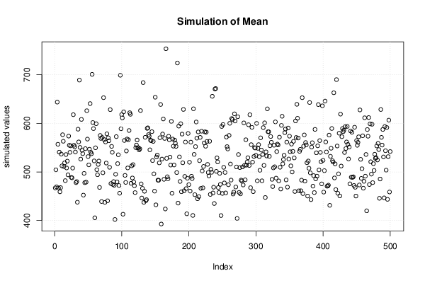
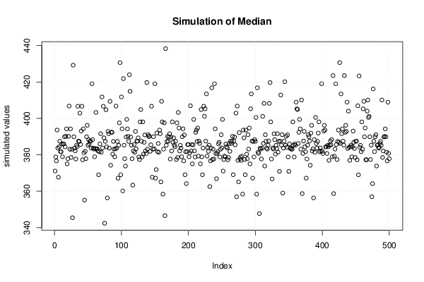
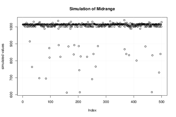
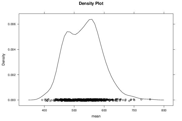
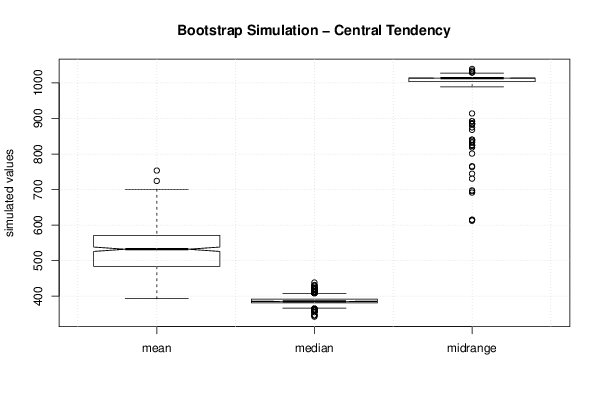
| Title produced by software | Blocked Bootstrap Plot - Central Tendency | ||||||||||||||||||||||||||||||||||||||||||||||||||||||||||||||||||||||||||||||||
| Date of computation | Sun, 16 Dec 2012 06:28:04 -0500 | ||||||||||||||||||||||||||||||||||||||||||||||||||||||||||||||||||||||||||||||||
| Cite this page as follows | Statistical Computations at FreeStatistics.org, Office for Research Development and Education, URL https://freestatistics.org/blog/index.php?v=date/2012/Dec/16/t1355657293wbk0qmdf9l4egow.htm/, Retrieved Sat, 12 Jul 2025 06:19:03 +0000 | ||||||||||||||||||||||||||||||||||||||||||||||||||||||||||||||||||||||||||||||||
| Statistical Computations at FreeStatistics.org, Office for Research Development and Education, URL https://freestatistics.org/blog/index.php?pk=200244, Retrieved Sat, 12 Jul 2025 06:19:03 +0000 | |||||||||||||||||||||||||||||||||||||||||||||||||||||||||||||||||||||||||||||||||
| QR Codes: | |||||||||||||||||||||||||||||||||||||||||||||||||||||||||||||||||||||||||||||||||
|
| |||||||||||||||||||||||||||||||||||||||||||||||||||||||||||||||||||||||||||||||||
| Original text written by user: | |||||||||||||||||||||||||||||||||||||||||||||||||||||||||||||||||||||||||||||||||
| IsPrivate? | No (this computation is public) | ||||||||||||||||||||||||||||||||||||||||||||||||||||||||||||||||||||||||||||||||
| User-defined keywords | |||||||||||||||||||||||||||||||||||||||||||||||||||||||||||||||||||||||||||||||||
| Estimated Impact | 187 | ||||||||||||||||||||||||||||||||||||||||||||||||||||||||||||||||||||||||||||||||
Tree of Dependent Computations | |||||||||||||||||||||||||||||||||||||||||||||||||||||||||||||||||||||||||||||||||
| Family? (F = Feedback message, R = changed R code, M = changed R Module, P = changed Parameters, D = changed Data) | |||||||||||||||||||||||||||||||||||||||||||||||||||||||||||||||||||||||||||||||||
| - [Bivariate Data Series] [Bivariate dataset] [2008-01-05 23:51:08] [74be16979710d4c4e7c6647856088456] - RMPD [Blocked Bootstrap Plot - Central Tendency] [Colombia Coffee] [2008-01-07 10:26:26] [74be16979710d4c4e7c6647856088456] - RM D [Blocked Bootstrap Plot - Central Tendency] [Paper] [2012-12-09 15:29:42] [9d44b52ac7f20a3e9be7c3c8470fe2cd] - D [Blocked Bootstrap Plot - Central Tendency] [paper] [2012-12-16 11:28:04] [97e5c69206415429213a02c19f23a896] [Current] | |||||||||||||||||||||||||||||||||||||||||||||||||||||||||||||||||||||||||||||||||
| Feedback Forum | |||||||||||||||||||||||||||||||||||||||||||||||||||||||||||||||||||||||||||||||||
Post a new message | |||||||||||||||||||||||||||||||||||||||||||||||||||||||||||||||||||||||||||||||||
Dataset | |||||||||||||||||||||||||||||||||||||||||||||||||||||||||||||||||||||||||||||||||
| Dataseries X: | |||||||||||||||||||||||||||||||||||||||||||||||||||||||||||||||||||||||||||||||||
414.89 444.50 481.29 491.09 419.70 432.88 438.01 412.84 402.91 416.20 411.80 393.60 381.70 388.34 370.89 385.96 394.26 381.37 377.40 377.70 347.71 347.70 340.20 341.00 342.00 319.54 302.79 299.10 313.50 326.80 316.00 316.50 317.20 330.40 323.35 325.85 321.50 321.90 347.48 338.89 345.70 340.44 342.40 342.70 348.34 376.66 417.73 423.51 397.56 390.92 408.26 401.12 408.91 438.35 460.23 449.59 450.52 461.15 460.38 465.35 467.57 486.24 476.58 442.07 443.61 451.55 451.07 451.33 437.63 431.28 413.46 406.78 420.17 419.05 404.01 387.51 390.15 384.40 371.05 367.60 375.04 365.14 361.75 366.88 394.26 409.39 410.11 416.81 393.06 374.24 369.05 352.33 362.53 394.73 389.32 380.74 381.73 376.95 383.64 363.83 363.34 358.38 356.95 366.72 367.69 356.31 348.74 358.69 360.17 361.73 354.45 353.91 344.34 338.62 337.24 340.81 352.72 343.06 345.43 344.38 335.02 334.82 329.01 329.31 330.08 342.15 367.18 371.89 392.19 378.84 355.28 364.18 373.83 383.30 386.88 381.91 384.13 377.27 381.43 385.64 385.49 380.36 391.58 389.77 384.39 379.29 378.55 376.64 382.12 391.03 385.22 387.56 386.23 383.67 383.06 383.14 385.31 387.44 399.45 404.76 396.21 392.85 391.93 385.27 383.47 387.35 383.14 381.07 377.85 369.00 355.11 346.58 351.81 344.47 343.84 340.76 324.10 324.01 322.82 324.87 306.04 288.74 289.10 297.49 295.94 308.29 299.10 292.32 292.87 284.11 288.98 295.93 294.12 291.68 287.08 287.33 285.96 282.62 276.44 261.31 256.08 256.69 264.74 310.72 293.18 283.07 284.32 299.86 286.39 279.69 275.19 285.73 281.59 274.47 273.68 270.00 266.01 271.45 265.49 261.87 263.03 260.48 272.36 270.23 267.53 272.39 283.42 283.06 276.16 275.85 281.51 295.50 294.06 302.68 314.49 321.18 313.29 310.26 319.14 316.56 319.07 331.92 356.86 358.97 340.55 328.18 355.68 356.35 351.02 359.77 378.95 378.92 389.91 406.95 413.79 404.88 406.67 403.26 383.78 392.37 398.09 400.51 405.28 420.46 439.38 442.08 424.03 423.35 433.85 429.23 421.87 430.66 424.48 437.93 456.05 469.90 476.67 510.10 549.86 555.00 557.09 610.65 675.39 596.15 633.71 632.59 598.19 585.78 627.83 629.79 631.17 664.75 654.90 679.37 667.31 655.66 665.38 665.41 712.65 754.60 806.25 803.20 889.60 922.30 968.43 909.71 888.66 889.49 939.77 839.03 829.93 806.62 760.86 816.09 858.69 943.00 924.27 890.20 928.65 945.67 934.23 949.38 996.59 1043.16 1127.04 1134.72 1117.96 1095.41 1113.34 1148.69 1205.43 1232.92 1192.97 1215.81 1270.98 1342.02 1369.89 1390.55 1356.40 1372.73 1424.00 1479.76 1512.60 1528.66 1572.21 1757.21 1770.95 1665.21 1738.11 1641.84 1652.21 1742.14 1673.77 1649.69 1591.19 1598.76 1589.90 1630.31 1744.81 1746.58 1721.64 | |||||||||||||||||||||||||||||||||||||||||||||||||||||||||||||||||||||||||||||||||
Tables (Output of Computation) | |||||||||||||||||||||||||||||||||||||||||||||||||||||||||||||||||||||||||||||||||
| |||||||||||||||||||||||||||||||||||||||||||||||||||||||||||||||||||||||||||||||||
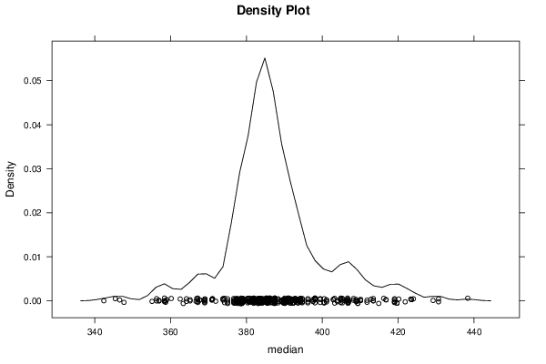
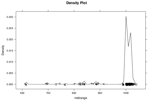
Figures (Output of Computation) | |||||||||||||||||||||||||||||||||||||||||||||||||||||||||||||||||||||||||||||||||
Input Parameters & R Code | |||||||||||||||||||||||||||||||||||||||||||||||||||||||||||||||||||||||||||||||||
| Parameters (Session): | |||||||||||||||||||||||||||||||||||||||||||||||||||||||||||||||||||||||||||||||||
| par1 = 500 ; par2 = 12 ; | |||||||||||||||||||||||||||||||||||||||||||||||||||||||||||||||||||||||||||||||||
| Parameters (R input): | |||||||||||||||||||||||||||||||||||||||||||||||||||||||||||||||||||||||||||||||||
| par1 = 500 ; par2 = 12 ; | |||||||||||||||||||||||||||||||||||||||||||||||||||||||||||||||||||||||||||||||||
| R code (references can be found in the software module): | |||||||||||||||||||||||||||||||||||||||||||||||||||||||||||||||||||||||||||||||||
par1 <- as.numeric(par1) | |||||||||||||||||||||||||||||||||||||||||||||||||||||||||||||||||||||||||||||||||