Free Statistics
of Irreproducible Research!
Description of Statistical Computation | |||||||||||||||||||||||||||||||||||||||||||||||||||||||||||||
|---|---|---|---|---|---|---|---|---|---|---|---|---|---|---|---|---|---|---|---|---|---|---|---|---|---|---|---|---|---|---|---|---|---|---|---|---|---|---|---|---|---|---|---|---|---|---|---|---|---|---|---|---|---|---|---|---|---|---|---|---|---|
| Author's title | |||||||||||||||||||||||||||||||||||||||||||||||||||||||||||||
| Author | *Unverified author* | ||||||||||||||||||||||||||||||||||||||||||||||||||||||||||||
| R Software Module | rwasp_linear_regression.wasp | ||||||||||||||||||||||||||||||||||||||||||||||||||||||||||||
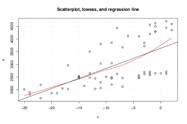
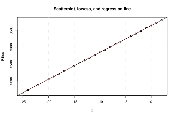
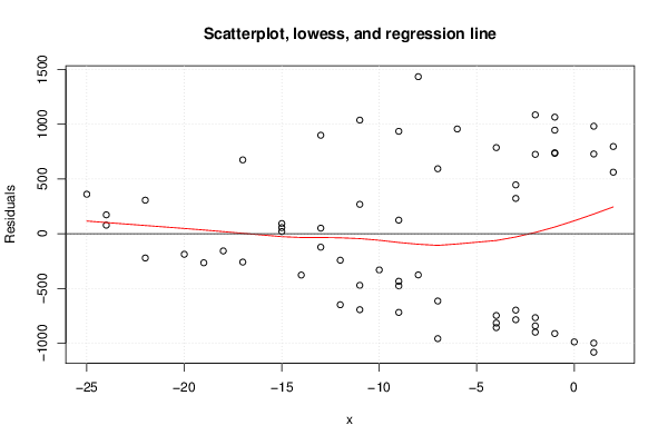
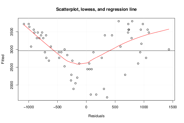
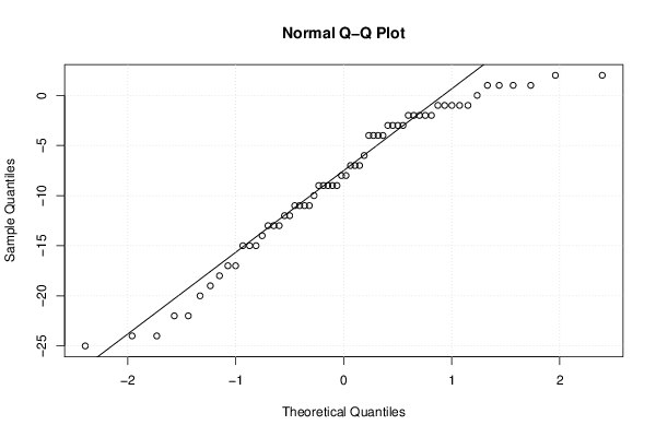
| Title produced by software | Linear Regression Graphical Model Validation | ||||||||||||||||||||||||||||||||||||||||||||||||||||||||||||
| Date of computation | Sun, 16 Dec 2012 04:53:30 -0500 | ||||||||||||||||||||||||||||||||||||||||||||||||||||||||||||
| Cite this page as follows | Statistical Computations at FreeStatistics.org, Office for Research Development and Education, URL https://freestatistics.org/blog/index.php?v=date/2012/Dec/16/t13556516979vfkrlt3vba4h1g.htm/, Retrieved Thu, 25 Apr 2024 21:26:50 +0000 | ||||||||||||||||||||||||||||||||||||||||||||||||||||||||||||
| Statistical Computations at FreeStatistics.org, Office for Research Development and Education, URL https://freestatistics.org/blog/index.php?pk=200196, Retrieved Thu, 25 Apr 2024 21:26:50 +0000 | |||||||||||||||||||||||||||||||||||||||||||||||||||||||||||||
| QR Codes: | |||||||||||||||||||||||||||||||||||||||||||||||||||||||||||||
|
| |||||||||||||||||||||||||||||||||||||||||||||||||||||||||||||
| Original text written by user: | |||||||||||||||||||||||||||||||||||||||||||||||||||||||||||||
| IsPrivate? | No (this computation is public) | ||||||||||||||||||||||||||||||||||||||||||||||||||||||||||||
| User-defined keywords | Simple Linear Regression Model Belgostat BEL-20 Inflation | ||||||||||||||||||||||||||||||||||||||||||||||||||||||||||||
| Estimated Impact | 132 | ||||||||||||||||||||||||||||||||||||||||||||||||||||||||||||
Tree of Dependent Computations | |||||||||||||||||||||||||||||||||||||||||||||||||||||||||||||
| Family? (F = Feedback message, R = changed R code, M = changed R Module, P = changed Parameters, D = changed Data) | |||||||||||||||||||||||||||||||||||||||||||||||||||||||||||||
| - [Bivariate Data Series] [Bivariate dataset] [2008-01-05 23:51:08] [74be16979710d4c4e7c6647856088456] F RMPD [Mean Plot] [Colombia Coffee] [2008-01-07 13:38:24] [74be16979710d4c4e7c6647856088456] - MPD [Mean Plot] [] [2011-12-21 12:12:27] [0cacbd6f25ea662f229a505efea21410] - RM D [Linear Regression Graphical Model Validation] [] [2011-12-21 13:11:38] [0cacbd6f25ea662f229a505efea21410] - R P [Linear Regression Graphical Model Validation] [Simple Linear Reg...] [2012-12-16 09:53:30] [d41d8cd98f00b204e9800998ecf8427e] [Current] | |||||||||||||||||||||||||||||||||||||||||||||||||||||||||||||
| Feedback Forum | |||||||||||||||||||||||||||||||||||||||||||||||||||||||||||||
Post a new message | |||||||||||||||||||||||||||||||||||||||||||||||||||||||||||||
Dataset | |||||||||||||||||||||||||||||||||||||||||||||||||||||||||||||
| Dataseries X: | |||||||||||||||||||||||||||||||||||||||||||||||||||||||||||||
-1 1 -1 2 2 1 -1 -2 -2 -1 -8 -4 -6 -3 -3 -7 -9 -11 -13 -11 -9 -17 -22 -25 -20 -24 -24 -22 -19 -18 -17 -11 -11 -12 -10 -15 -15 -15 -13 -8 -13 -9 -7 -4 -4 -2 0 -2 -3 1 -2 -1 1 -3 -4 -9 -9 -7 -14 -12 | |||||||||||||||||||||||||||||||||||||||||||||||||||||||||||||
| Dataseries Y: | |||||||||||||||||||||||||||||||||||||||||||||||||||||||||||||
4290.89 4443.91 4502.64 4356.98 4591.27 4696.96 4621.4 4562.84 4202.52 4296.49 4435.23 4105.18 4116.68 3844.49 3720.98 3674.4 3857.62 3801.06 3504.37 3032.6 3047.03 2962.34 2197.82 2014.45 1862.83 1905.41 1810.99 1670.07 1864.44 2052.02 2029.6 2070.83 2293.41 2443.27 2513.17 2466.92 2502.66 2539.91 2482.6 2626.15 2656.32 2446.66 2467.38 2462.32 2504.58 2579.39 2649.24 2636.87 2613.94 2634.01 2711.94 2646.43 2717.79 2701.54 2572.98 2488.92 2204.91 2123.99 2149.1 2036.71 | |||||||||||||||||||||||||||||||||||||||||||||||||||||||||||||
Tables (Output of Computation) | |||||||||||||||||||||||||||||||||||||||||||||||||||||||||||||
| |||||||||||||||||||||||||||||||||||||||||||||||||||||||||||||
Figures (Output of Computation) | |||||||||||||||||||||||||||||||||||||||||||||||||||||||||||||
Input Parameters & R Code | |||||||||||||||||||||||||||||||||||||||||||||||||||||||||||||
| Parameters (Session): | |||||||||||||||||||||||||||||||||||||||||||||||||||||||||||||
| par1 = 0 ; | |||||||||||||||||||||||||||||||||||||||||||||||||||||||||||||
| Parameters (R input): | |||||||||||||||||||||||||||||||||||||||||||||||||||||||||||||
| par1 = 0 ; | |||||||||||||||||||||||||||||||||||||||||||||||||||||||||||||
| R code (references can be found in the software module): | |||||||||||||||||||||||||||||||||||||||||||||||||||||||||||||
par1 <- as.numeric(par1) | |||||||||||||||||||||||||||||||||||||||||||||||||||||||||||||