Free Statistics
of Irreproducible Research!
Description of Statistical Computation | |||||||||||||||||||||
|---|---|---|---|---|---|---|---|---|---|---|---|---|---|---|---|---|---|---|---|---|---|
| Author's title | |||||||||||||||||||||
| Author | *The author of this computation has been verified* | ||||||||||||||||||||
| R Software Module | rwasp_meanplot.wasp | ||||||||||||||||||||
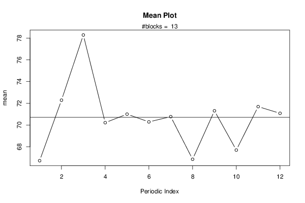
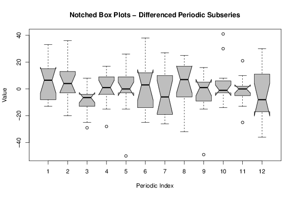
| Title produced by software | Mean Plot | ||||||||||||||||||||
| Date of computation | Fri, 14 Dec 2012 07:38:16 -0500 | ||||||||||||||||||||
| Cite this page as follows | Statistical Computations at FreeStatistics.org, Office for Research Development and Education, URL https://freestatistics.org/blog/index.php?v=date/2012/Dec/14/t1355488717vx2t9op6vxtg7hw.htm/, Retrieved Thu, 25 Apr 2024 13:44:12 +0000 | ||||||||||||||||||||
| Statistical Computations at FreeStatistics.org, Office for Research Development and Education, URL https://freestatistics.org/blog/index.php?pk=199523, Retrieved Thu, 25 Apr 2024 13:44:12 +0000 | |||||||||||||||||||||
| QR Codes: | |||||||||||||||||||||
|
| |||||||||||||||||||||
| Original text written by user: | |||||||||||||||||||||
| IsPrivate? | No (this computation is public) | ||||||||||||||||||||
| User-defined keywords | |||||||||||||||||||||
| Estimated Impact | 92 | ||||||||||||||||||||
Tree of Dependent Computations | |||||||||||||||||||||
| Family? (F = Feedback message, R = changed R code, M = changed R Module, P = changed Parameters, D = changed Data) | |||||||||||||||||||||
| - [Mean Plot] [] [2011-11-17 21:14:10] [a2638725f7f7c6bd63902ba17eba666b] - R [Mean Plot] [Paper deel 3] [2012-12-14 12:38:16] [413ae3079a2d7d57ac33b6b2184bdf0e] [Current] | |||||||||||||||||||||
| Feedback Forum | |||||||||||||||||||||
Post a new message | |||||||||||||||||||||
Dataset | |||||||||||||||||||||
| Dataseries X: | |||||||||||||||||||||
53 86 66 67 76 78 53 80 74 76 79 54 67 54 87 58 75 88 64 57 66 68 54 56 86 80 76 69 78 67 80 54 71 84 74 71 63 71 76 69 74 75 54 52 69 68 65 75 74 75 72 67 63 62 63 76 74 67 73 70 53 77 77 52 54 80 66 73 63 69 67 54 81 69 84 80 70 69 77 54 79 30 71 73 72 77 75 69 54 70 73 54 77 82 80 80 69 78 81 76 76 73 85 66 79 68 76 71 54 46 82 74 88 38 76 86 54 70 69 90 54 76 89 76 73 79 90 74 81 72 71 66 77 65 74 82 54 63 54 64 69 54 84 86 77 89 76 60 75 73 85 79 71 72 69 78 54 69 81 84 84 69 | |||||||||||||||||||||
Tables (Output of Computation) | |||||||||||||||||||||
| |||||||||||||||||||||
Figures (Output of Computation) | |||||||||||||||||||||
Input Parameters & R Code | |||||||||||||||||||||
| Parameters (Session): | |||||||||||||||||||||
| par1 = 12 ; | |||||||||||||||||||||
| Parameters (R input): | |||||||||||||||||||||
| par1 = 12 ; | |||||||||||||||||||||
| R code (references can be found in the software module): | |||||||||||||||||||||
par1 <- as.numeric(par1) | |||||||||||||||||||||