Free Statistics
of Irreproducible Research!
Description of Statistical Computation | |||||||||||||||||||||
|---|---|---|---|---|---|---|---|---|---|---|---|---|---|---|---|---|---|---|---|---|---|
| Author's title | |||||||||||||||||||||
| Author | *Unverified author* | ||||||||||||||||||||
| R Software Module | rwasp_sdplot.wasp | ||||||||||||||||||||
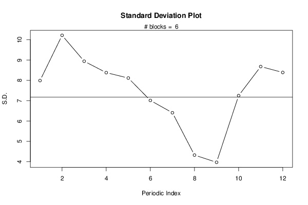
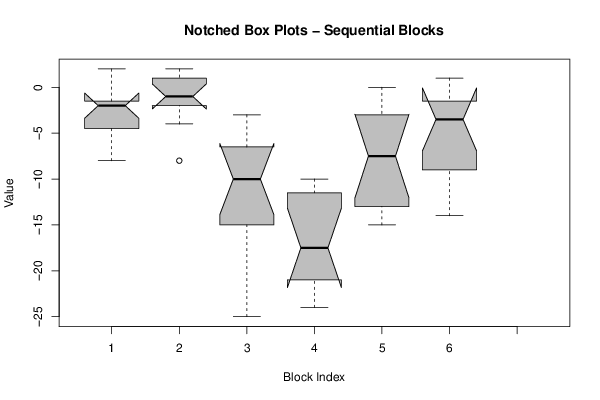
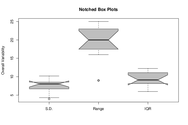
| Title produced by software | Standard Deviation Plot | ||||||||||||||||||||
| Date of computation | Thu, 13 Dec 2012 13:51:07 -0500 | ||||||||||||||||||||
| Cite this page as follows | Statistical Computations at FreeStatistics.org, Office for Research Development and Education, URL https://freestatistics.org/blog/index.php?v=date/2012/Dec/13/t1355424684rvxkvoi9cihdigc.htm/, Retrieved Sun, 28 Apr 2024 20:22:16 +0000 | ||||||||||||||||||||
| Statistical Computations at FreeStatistics.org, Office for Research Development and Education, URL https://freestatistics.org/blog/index.php?pk=199362, Retrieved Sun, 28 Apr 2024 20:22:16 +0000 | |||||||||||||||||||||
| QR Codes: | |||||||||||||||||||||
|
| |||||||||||||||||||||
| Original text written by user: | |||||||||||||||||||||
| IsPrivate? | No (this computation is public) | ||||||||||||||||||||
| User-defined keywords | |||||||||||||||||||||
| Estimated Impact | 108 | ||||||||||||||||||||
Tree of Dependent Computations | |||||||||||||||||||||
| Family? (F = Feedback message, R = changed R code, M = changed R Module, P = changed Parameters, D = changed Data) | |||||||||||||||||||||
| - [Standard Deviation Plot] [] [2012-12-13 18:51:07] [0769c782addd77dfcec38b8d0e028078] [Current] - RMP [Classical Decomposition] [] [2012-12-29 13:48:32] [443e3dc6fee66d7ac3a3c54fbf520d20] - RMPD [Exponential Smoothing] [] [2012-12-29 14:03:59] [8adb8cce9eee629aacf8316cc643cd55] - RMP [Exponential Smoothing] [] [2012-12-29 14:10:45] [8adb8cce9eee629aacf8316cc643cd55] | |||||||||||||||||||||
| Feedback Forum | |||||||||||||||||||||
Post a new message | |||||||||||||||||||||
Dataset | |||||||||||||||||||||
| Dataseries X: | |||||||||||||||||||||
-1 -2 -5 -4 -6 -2 -2 -2 -2 2 1 -8 -1 1 -1 2 2 1 -1 -2 -2 -1 -8 -4 -6 -3 -3 -7 -9 -11 -13 -11 -9 -17 -22 -25 -20 -24 -24 -22 -19 -18 -17 -11 -11 -12 -10 -15 -15 -15 -13 -8 -13 -9 -7 -4 -4 -2 0 -2 -3 1 -2 -1 1 -3 -4 -9 -9 -7 -14 -12 | |||||||||||||||||||||
Tables (Output of Computation) | |||||||||||||||||||||
| |||||||||||||||||||||
Figures (Output of Computation) | |||||||||||||||||||||
Input Parameters & R Code | |||||||||||||||||||||
| Parameters (Session): | |||||||||||||||||||||
| par1 = 12 ; | |||||||||||||||||||||
| Parameters (R input): | |||||||||||||||||||||
| par1 = 12 ; | |||||||||||||||||||||
| R code (references can be found in the software module): | |||||||||||||||||||||
par1 <- as.numeric(par1) | |||||||||||||||||||||