Repository of Reproducible Computations

Free Statistics

of Irreproducible Research!

Author's title

Author

*The author of this computation has been verified*

R Software Module

rwasp_autocorrelation.wasp

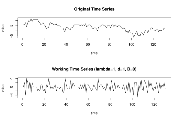
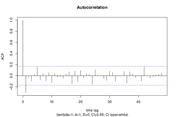
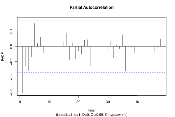
Title produced by software

(Partial) Autocorrelation Function

Date of computation

Thu, 13 Dec 2012 09:23:27 -0500

Cite this page as follows

Statistical Computations at FreeStatistics.org, Office for Research Development and Education, URL https://freestatistics.org/blog/index.php?v=date/2012/Dec/13/t1355408635hs6wyvctop2kk5i.htm/, Retrieved Sun, 28 Apr 2024 23:48:30 +0000

Statistical Computations at FreeStatistics.org, Office for Research Development and Education, URL https://freestatistics.org/blog/index.php?pk=199247, Retrieved Sun, 28 Apr 2024 23:48:30 +0000

QR Codes:

Paste this QR Code to cite your computation.

Original text written by user:

IsPrivate?

No (this computation is public)

User-defined keywords

Estimated Impact

130

Family? (F = Feedback message, R = changed R code, M = changed R Module, P = changed Parameters, D = changed Data)

-     [Univariate Data Series] [data set] [2008-12-01 19:54:57] [b98453cac15ba1066b407e146608df68]
- RMP   [(Partial) Autocorrelation Function] [Unemployment] [2010-11-29 09:09:37] [b98453cac15ba1066b407e146608df68]
-    D    [(Partial) Autocorrelation Function] [] [2010-12-15 16:30:30] [8d263c682820d5327cb5f02a8c3630cf]
-   PD      [(Partial) Autocorrelation Function] [] [2010-12-17 08:16:08] [4dfa50539945b119a90a7606969443b9]
- R           [(Partial) Autocorrelation Function] [] [2010-12-17 11:19:45] [c6813a60da787bb62b5d86150b8926dd]
-   PD          [(Partial) Autocorrelation Function] [] [2010-12-27 20:40:18] [c6813a60da787bb62b5d86150b8926dd]
- R P               [(Partial) Autocorrelation Function] [Deel 4: ARIMA aut...] [2012-12-13 14:23:27] [f988ca26b10d35edf58465884f70a009] [Current]

Feedback Forum

Post a new message

Dataseries X:

Download CSV

Histogram

Boxplots

Summary of computational transaction
Raw Input	view raw input (R code)
Raw Output	view raw output of R engine
Computing time	3 seconds
R Server	'Gwilym Jenkins' @ jenkins.wessa.net

\begin{tabular}{lllllllll}
\hline
Summary of computational transaction \tabularnewline
Raw Input & view raw input (R code)  \tabularnewline
Raw Output & view raw output of R engine  \tabularnewline
Computing time & 3 seconds \tabularnewline
R Server & 'Gwilym Jenkins' @ jenkins.wessa.net \tabularnewline
\hline
\end{tabular}
%Source: https://freestatistics.org/blog/index.php?pk=199247&T=0

[TABLE]
[ROW][C]Summary of computational transaction[/C][/ROW]
[ROW][C]Raw Input[/C][C]view raw input (R code) [/C][/ROW]
[ROW][C]Raw Output[/C][C]view raw output of R engine [/C][/ROW]
[ROW][C]Computing time[/C][C]3 seconds[/C][/ROW]
[ROW][C]R Server[/C][C]'Gwilym Jenkins' @ jenkins.wessa.net[/C][/ROW]
[/TABLE]
Source: https://freestatistics.org/blog/index.php?pk=199247&T=0

Globally Unique Identifier (entire table): ba.freestatistics.org/blog/index.php?pk=199247&T=0

As an alternative you can also use a QR Code:

The GUIDs for individual cells are displayed in the table below:

Summary of computational transaction
Raw Input	view raw input (R code)
Raw Output	view raw output of R engine
Computing time	3 seconds
R Server	'Gwilym Jenkins' @ jenkins.wessa.net

Autocorrelation Function
Time lag k	ACF(k)	T-STAT	P-value
1	-0.303627	-3.4619	0.000363
2	-0.024219	-0.2761	0.391442
3	-0.09504	-1.0836	0.140269
4	0.027852	0.3176	0.375664
5	0.162887	1.8572	0.032773
6	-0.078965	-0.9003	0.184803
7	0.039551	0.451	0.326388
8	-0.095343	-1.0871	0.139507
9	0.056066	0.6393	0.261892
10	-0.12401	-1.4139	0.079885
11	0.039542	0.4508	0.326425
12	-0.024314	-0.2772	0.391025
13	-0.019576	-0.2232	0.411867
14	-0.045652	-0.5205	0.301797
15	0.035011	0.3992	0.345204
16	0.072862	0.8308	0.203818
17	-0.145068	-1.654	0.050267
18	0.084782	0.9667	0.167754
19	-0.102479	-1.1684	0.122385
20	0.096483	1.1001	0.136665
21	-0.031154	-0.3552	0.361506
22	0.042325	0.4826	0.315102
23	0.025439	0.29	0.386121
24	-0.152559	-1.7394	0.042162
25	0.108032	1.2318	0.110132
26	0.004172	0.0476	0.481067
27	0.001653	0.0189	0.492494
28	-0.05057	-0.5766	0.282609
29	-0.086273	-0.9837	0.163553
30	0.079868	0.9106	0.182085
31	0.061049	0.6961	0.243814
32	-0.100137	-1.1417	0.12783
33	0.004375	0.0499	0.480147
34	0.001856	0.0212	0.491573
35	0.080222	0.9147	0.181029
36	-0.137926	-1.5726	0.059121
37	0.073471	0.8377	0.201869
38	0.033391	0.3807	0.352016
39	-0.030975	-0.3532	0.362266
40	0.006948	0.0792	0.468488
41	-0.099574	-1.1353	0.129165
42	0.158939	1.8122	0.036133
43	-0.004545	-0.0518	0.479373
44	-0.038024	-0.4335	0.332668
45	-0.014177	-0.1616	0.435918
46	0.016562	0.1888	0.425257
47	0.028193	0.3214	0.374193
48	0.04967	0.5663	0.286075

\begin{tabular}{lllllllll}
\hline
Autocorrelation Function \tabularnewline
Time lag k & ACF(k) & T-STAT & P-value \tabularnewline
1 & -0.303627 & -3.4619 & 0.000363 \tabularnewline
2 & -0.024219 & -0.2761 & 0.391442 \tabularnewline
3 & -0.09504 & -1.0836 & 0.140269 \tabularnewline
4 & 0.027852 & 0.3176 & 0.375664 \tabularnewline
5 & 0.162887 & 1.8572 & 0.032773 \tabularnewline
6 & -0.078965 & -0.9003 & 0.184803 \tabularnewline
7 & 0.039551 & 0.451 & 0.326388 \tabularnewline
8 & -0.095343 & -1.0871 & 0.139507 \tabularnewline
9 & 0.056066 & 0.6393 & 0.261892 \tabularnewline
10 & -0.12401 & -1.4139 & 0.079885 \tabularnewline
11 & 0.039542 & 0.4508 & 0.326425 \tabularnewline
12 & -0.024314 & -0.2772 & 0.391025 \tabularnewline
13 & -0.019576 & -0.2232 & 0.411867 \tabularnewline
14 & -0.045652 & -0.5205 & 0.301797 \tabularnewline
15 & 0.035011 & 0.3992 & 0.345204 \tabularnewline
16 & 0.072862 & 0.8308 & 0.203818 \tabularnewline
17 & -0.145068 & -1.654 & 0.050267 \tabularnewline
18 & 0.084782 & 0.9667 & 0.167754 \tabularnewline
19 & -0.102479 & -1.1684 & 0.122385 \tabularnewline
20 & 0.096483 & 1.1001 & 0.136665 \tabularnewline
21 & -0.031154 & -0.3552 & 0.361506 \tabularnewline
22 & 0.042325 & 0.4826 & 0.315102 \tabularnewline
23 & 0.025439 & 0.29 & 0.386121 \tabularnewline
24 & -0.152559 & -1.7394 & 0.042162 \tabularnewline
25 & 0.108032 & 1.2318 & 0.110132 \tabularnewline
26 & 0.004172 & 0.0476 & 0.481067 \tabularnewline
27 & 0.001653 & 0.0189 & 0.492494 \tabularnewline
28 & -0.05057 & -0.5766 & 0.282609 \tabularnewline
29 & -0.086273 & -0.9837 & 0.163553 \tabularnewline
30 & 0.079868 & 0.9106 & 0.182085 \tabularnewline
31 & 0.061049 & 0.6961 & 0.243814 \tabularnewline
32 & -0.100137 & -1.1417 & 0.12783 \tabularnewline
33 & 0.004375 & 0.0499 & 0.480147 \tabularnewline
34 & 0.001856 & 0.0212 & 0.491573 \tabularnewline
35 & 0.080222 & 0.9147 & 0.181029 \tabularnewline
36 & -0.137926 & -1.5726 & 0.059121 \tabularnewline
37 & 0.073471 & 0.8377 & 0.201869 \tabularnewline
38 & 0.033391 & 0.3807 & 0.352016 \tabularnewline
39 & -0.030975 & -0.3532 & 0.362266 \tabularnewline
40 & 0.006948 & 0.0792 & 0.468488 \tabularnewline
41 & -0.099574 & -1.1353 & 0.129165 \tabularnewline
42 & 0.158939 & 1.8122 & 0.036133 \tabularnewline
43 & -0.004545 & -0.0518 & 0.479373 \tabularnewline
44 & -0.038024 & -0.4335 & 0.332668 \tabularnewline
45 & -0.014177 & -0.1616 & 0.435918 \tabularnewline
46 & 0.016562 & 0.1888 & 0.425257 \tabularnewline
47 & 0.028193 & 0.3214 & 0.374193 \tabularnewline
48 & 0.04967 & 0.5663 & 0.286075 \tabularnewline
\hline
\end{tabular}
%Source: https://freestatistics.org/blog/index.php?pk=199247&T=1

[TABLE]
[ROW][C]Autocorrelation Function[/C][/ROW]
[ROW][C]Time lag k[/C][C]ACF(k)[/C][C]T-STAT[/C][C]P-value[/C][/ROW]
[ROW][C]1[/C][C]-0.303627[/C][C]-3.4619[/C][C]0.000363[/C][/ROW]
[ROW][C]2[/C][C]-0.024219[/C][C]-0.2761[/C][C]0.391442[/C][/ROW]
[ROW][C]3[/C][C]-0.09504[/C][C]-1.0836[/C][C]0.140269[/C][/ROW]
[ROW][C]4[/C][C]0.027852[/C][C]0.3176[/C][C]0.375664[/C][/ROW]
[ROW][C]5[/C][C]0.162887[/C][C]1.8572[/C][C]0.032773[/C][/ROW]
[ROW][C]6[/C][C]-0.078965[/C][C]-0.9003[/C][C]0.184803[/C][/ROW]
[ROW][C]7[/C][C]0.039551[/C][C]0.451[/C][C]0.326388[/C][/ROW]
[ROW][C]8[/C][C]-0.095343[/C][C]-1.0871[/C][C]0.139507[/C][/ROW]
[ROW][C]9[/C][C]0.056066[/C][C]0.6393[/C][C]0.261892[/C][/ROW]
[ROW][C]10[/C][C]-0.12401[/C][C]-1.4139[/C][C]0.079885[/C][/ROW]
[ROW][C]11[/C][C]0.039542[/C][C]0.4508[/C][C]0.326425[/C][/ROW]
[ROW][C]12[/C][C]-0.024314[/C][C]-0.2772[/C][C]0.391025[/C][/ROW]
[ROW][C]13[/C][C]-0.019576[/C][C]-0.2232[/C][C]0.411867[/C][/ROW]
[ROW][C]14[/C][C]-0.045652[/C][C]-0.5205[/C][C]0.301797[/C][/ROW]
[ROW][C]15[/C][C]0.035011[/C][C]0.3992[/C][C]0.345204[/C][/ROW]
[ROW][C]16[/C][C]0.072862[/C][C]0.8308[/C][C]0.203818[/C][/ROW]
[ROW][C]17[/C][C]-0.145068[/C][C]-1.654[/C][C]0.050267[/C][/ROW]
[ROW][C]18[/C][C]0.084782[/C][C]0.9667[/C][C]0.167754[/C][/ROW]
[ROW][C]19[/C][C]-0.102479[/C][C]-1.1684[/C][C]0.122385[/C][/ROW]
[ROW][C]20[/C][C]0.096483[/C][C]1.1001[/C][C]0.136665[/C][/ROW]
[ROW][C]21[/C][C]-0.031154[/C][C]-0.3552[/C][C]0.361506[/C][/ROW]
[ROW][C]22[/C][C]0.042325[/C][C]0.4826[/C][C]0.315102[/C][/ROW]
[ROW][C]23[/C][C]0.025439[/C][C]0.29[/C][C]0.386121[/C][/ROW]
[ROW][C]24[/C][C]-0.152559[/C][C]-1.7394[/C][C]0.042162[/C][/ROW]
[ROW][C]25[/C][C]0.108032[/C][C]1.2318[/C][C]0.110132[/C][/ROW]
[ROW][C]26[/C][C]0.004172[/C][C]0.0476[/C][C]0.481067[/C][/ROW]
[ROW][C]27[/C][C]0.001653[/C][C]0.0189[/C][C]0.492494[/C][/ROW]
[ROW][C]28[/C][C]-0.05057[/C][C]-0.5766[/C][C]0.282609[/C][/ROW]
[ROW][C]29[/C][C]-0.086273[/C][C]-0.9837[/C][C]0.163553[/C][/ROW]
[ROW][C]30[/C][C]0.079868[/C][C]0.9106[/C][C]0.182085[/C][/ROW]
[ROW][C]31[/C][C]0.061049[/C][C]0.6961[/C][C]0.243814[/C][/ROW]
[ROW][C]32[/C][C]-0.100137[/C][C]-1.1417[/C][C]0.12783[/C][/ROW]
[ROW][C]33[/C][C]0.004375[/C][C]0.0499[/C][C]0.480147[/C][/ROW]
[ROW][C]34[/C][C]0.001856[/C][C]0.0212[/C][C]0.491573[/C][/ROW]
[ROW][C]35[/C][C]0.080222[/C][C]0.9147[/C][C]0.181029[/C][/ROW]
[ROW][C]36[/C][C]-0.137926[/C][C]-1.5726[/C][C]0.059121[/C][/ROW]
[ROW][C]37[/C][C]0.073471[/C][C]0.8377[/C][C]0.201869[/C][/ROW]
[ROW][C]38[/C][C]0.033391[/C][C]0.3807[/C][C]0.352016[/C][/ROW]
[ROW][C]39[/C][C]-0.030975[/C][C]-0.3532[/C][C]0.362266[/C][/ROW]
[ROW][C]40[/C][C]0.006948[/C][C]0.0792[/C][C]0.468488[/C][/ROW]
[ROW][C]41[/C][C]-0.099574[/C][C]-1.1353[/C][C]0.129165[/C][/ROW]
[ROW][C]42[/C][C]0.158939[/C][C]1.8122[/C][C]0.036133[/C][/ROW]
[ROW][C]43[/C][C]-0.004545[/C][C]-0.0518[/C][C]0.479373[/C][/ROW]
[ROW][C]44[/C][C]-0.038024[/C][C]-0.4335[/C][C]0.332668[/C][/ROW]
[ROW][C]45[/C][C]-0.014177[/C][C]-0.1616[/C][C]0.435918[/C][/ROW]
[ROW][C]46[/C][C]0.016562[/C][C]0.1888[/C][C]0.425257[/C][/ROW]
[ROW][C]47[/C][C]0.028193[/C][C]0.3214[/C][C]0.374193[/C][/ROW]
[ROW][C]48[/C][C]0.04967[/C][C]0.5663[/C][C]0.286075[/C][/ROW]
[/TABLE]
Source: https://freestatistics.org/blog/index.php?pk=199247&T=1

Globally Unique Identifier (entire table): ba.freestatistics.org/blog/index.php?pk=199247&T=1

As an alternative you can also use a QR Code:

The GUIDs for individual cells are displayed in the table below:

Autocorrelation Function
Time lag k	ACF(k)	T-STAT	P-value
1	-0.303627	-3.4619	0.000363
2	-0.024219	-0.2761	0.391442
3	-0.09504	-1.0836	0.140269
4	0.027852	0.3176	0.375664
5	0.162887	1.8572	0.032773
6	-0.078965	-0.9003	0.184803
7	0.039551	0.451	0.326388
8	-0.095343	-1.0871	0.139507
9	0.056066	0.6393	0.261892
10	-0.12401	-1.4139	0.079885
11	0.039542	0.4508	0.326425
12	-0.024314	-0.2772	0.391025
13	-0.019576	-0.2232	0.411867
14	-0.045652	-0.5205	0.301797
15	0.035011	0.3992	0.345204
16	0.072862	0.8308	0.203818
17	-0.145068	-1.654	0.050267
18	0.084782	0.9667	0.167754
19	-0.102479	-1.1684	0.122385
20	0.096483	1.1001	0.136665
21	-0.031154	-0.3552	0.361506
22	0.042325	0.4826	0.315102
23	0.025439	0.29	0.386121
24	-0.152559	-1.7394	0.042162
25	0.108032	1.2318	0.110132
26	0.004172	0.0476	0.481067
27	0.001653	0.0189	0.492494
28	-0.05057	-0.5766	0.282609
29	-0.086273	-0.9837	0.163553
30	0.079868	0.9106	0.182085
31	0.061049	0.6961	0.243814
32	-0.100137	-1.1417	0.12783
33	0.004375	0.0499	0.480147
34	0.001856	0.0212	0.491573
35	0.080222	0.9147	0.181029
36	-0.137926	-1.5726	0.059121
37	0.073471	0.8377	0.201869
38	0.033391	0.3807	0.352016
39	-0.030975	-0.3532	0.362266
40	0.006948	0.0792	0.468488
41	-0.099574	-1.1353	0.129165
42	0.158939	1.8122	0.036133
43	-0.004545	-0.0518	0.479373
44	-0.038024	-0.4335	0.332668
45	-0.014177	-0.1616	0.435918
46	0.016562	0.1888	0.425257
47	0.028193	0.3214	0.374193
48	0.04967	0.5663	0.286075

Partial Autocorrelation Function
Time lag k	PACF(k)	T-STAT	P-value
1	-0.303627	-3.4619	0.000363
2	-0.128229	-1.462	0.073072
3	-0.159338	-1.8167	0.035781
4	-0.068321	-0.779	0.218705
5	0.149553	1.7052	0.045276
6	0.0181	0.2064	0.418411
7	0.059698	0.6807	0.248648
8	-0.041727	-0.4758	0.317523
9	0.004606	0.0525	0.479098
10	-0.162558	-1.8534	0.033043
11	-0.069773	-0.7955	0.213876
12	-0.075157	-0.8569	0.196533
13	-0.061347	-0.6995	0.242755
14	-0.096001	-1.0946	0.137862
15	0.032677	0.3726	0.355037
16	0.088878	1.0134	0.156384
17	-0.089839	-1.0243	0.153794
18	0.024566	0.2801	0.389926
19	-0.081005	-0.9236	0.178703
20	-0.029218	-0.3331	0.369785
21	-0.052959	-0.6038	0.273506
22	0.040415	0.4608	0.322855
23	0.04422	0.5042	0.307494
24	-0.127576	-1.4546	0.074096
25	0.008146	0.0929	0.463072
26	0.054452	0.6208	0.267893
27	-0.070652	-0.8056	0.210985
28	-0.0569	-0.6488	0.25882
29	-0.124255	-1.4167	0.079477
30	-0.027308	-0.3114	0.378012
31	0.034732	0.396	0.346376
32	-0.074478	-0.8492	0.198671
33	0.007274	0.0829	0.467014
34	-0.015305	-0.1745	0.43087
35	0.076745	0.875	0.191586
36	-0.159699	-1.8208	0.035465
37	0.000552	0.0063	0.497496
38	-0.002698	-0.0308	0.487754
39	-0.04087	-0.466	0.321
40	-0.024788	-0.2826	0.388954
41	-0.119392	-1.3613	0.087891
42	0.081795	0.9326	0.176377
43	0.044908	0.512	0.304749
44	-0.012365	-0.141	0.44405
45	0.016593	0.1892	0.425118
46	-0.037743	-0.4303	0.333833
47	-0.004851	-0.0553	0.477989
48	0.050131	0.5716	0.284296

\begin{tabular}{lllllllll}
\hline
Partial Autocorrelation Function \tabularnewline
Time lag k & PACF(k) & T-STAT & P-value \tabularnewline
1 & -0.303627 & -3.4619 & 0.000363 \tabularnewline
2 & -0.128229 & -1.462 & 0.073072 \tabularnewline
3 & -0.159338 & -1.8167 & 0.035781 \tabularnewline
4 & -0.068321 & -0.779 & 0.218705 \tabularnewline
5 & 0.149553 & 1.7052 & 0.045276 \tabularnewline
6 & 0.0181 & 0.2064 & 0.418411 \tabularnewline
7 & 0.059698 & 0.6807 & 0.248648 \tabularnewline
8 & -0.041727 & -0.4758 & 0.317523 \tabularnewline
9 & 0.004606 & 0.0525 & 0.479098 \tabularnewline
10 & -0.162558 & -1.8534 & 0.033043 \tabularnewline
11 & -0.069773 & -0.7955 & 0.213876 \tabularnewline
12 & -0.075157 & -0.8569 & 0.196533 \tabularnewline
13 & -0.061347 & -0.6995 & 0.242755 \tabularnewline
14 & -0.096001 & -1.0946 & 0.137862 \tabularnewline
15 & 0.032677 & 0.3726 & 0.355037 \tabularnewline
16 & 0.088878 & 1.0134 & 0.156384 \tabularnewline
17 & -0.089839 & -1.0243 & 0.153794 \tabularnewline
18 & 0.024566 & 0.2801 & 0.389926 \tabularnewline
19 & -0.081005 & -0.9236 & 0.178703 \tabularnewline
20 & -0.029218 & -0.3331 & 0.369785 \tabularnewline
21 & -0.052959 & -0.6038 & 0.273506 \tabularnewline
22 & 0.040415 & 0.4608 & 0.322855 \tabularnewline
23 & 0.04422 & 0.5042 & 0.307494 \tabularnewline
24 & -0.127576 & -1.4546 & 0.074096 \tabularnewline
25 & 0.008146 & 0.0929 & 0.463072 \tabularnewline
26 & 0.054452 & 0.6208 & 0.267893 \tabularnewline
27 & -0.070652 & -0.8056 & 0.210985 \tabularnewline
28 & -0.0569 & -0.6488 & 0.25882 \tabularnewline
29 & -0.124255 & -1.4167 & 0.079477 \tabularnewline
30 & -0.027308 & -0.3114 & 0.378012 \tabularnewline
31 & 0.034732 & 0.396 & 0.346376 \tabularnewline
32 & -0.074478 & -0.8492 & 0.198671 \tabularnewline
33 & 0.007274 & 0.0829 & 0.467014 \tabularnewline
34 & -0.015305 & -0.1745 & 0.43087 \tabularnewline
35 & 0.076745 & 0.875 & 0.191586 \tabularnewline
36 & -0.159699 & -1.8208 & 0.035465 \tabularnewline
37 & 0.000552 & 0.0063 & 0.497496 \tabularnewline
38 & -0.002698 & -0.0308 & 0.487754 \tabularnewline
39 & -0.04087 & -0.466 & 0.321 \tabularnewline
40 & -0.024788 & -0.2826 & 0.388954 \tabularnewline
41 & -0.119392 & -1.3613 & 0.087891 \tabularnewline
42 & 0.081795 & 0.9326 & 0.176377 \tabularnewline
43 & 0.044908 & 0.512 & 0.304749 \tabularnewline
44 & -0.012365 & -0.141 & 0.44405 \tabularnewline
45 & 0.016593 & 0.1892 & 0.425118 \tabularnewline
46 & -0.037743 & -0.4303 & 0.333833 \tabularnewline
47 & -0.004851 & -0.0553 & 0.477989 \tabularnewline
48 & 0.050131 & 0.5716 & 0.284296 \tabularnewline
\hline
\end{tabular}
%Source: https://freestatistics.org/blog/index.php?pk=199247&T=2

[TABLE]
[ROW][C]Partial Autocorrelation Function[/C][/ROW]
[ROW][C]Time lag k[/C][C]PACF(k)[/C][C]T-STAT[/C][C]P-value[/C][/ROW]
[ROW][C]1[/C][C]-0.303627[/C][C]-3.4619[/C][C]0.000363[/C][/ROW]
[ROW][C]2[/C][C]-0.128229[/C][C]-1.462[/C][C]0.073072[/C][/ROW]
[ROW][C]3[/C][C]-0.159338[/C][C]-1.8167[/C][C]0.035781[/C][/ROW]
[ROW][C]4[/C][C]-0.068321[/C][C]-0.779[/C][C]0.218705[/C][/ROW]
[ROW][C]5[/C][C]0.149553[/C][C]1.7052[/C][C]0.045276[/C][/ROW]
[ROW][C]6[/C][C]0.0181[/C][C]0.2064[/C][C]0.418411[/C][/ROW]
[ROW][C]7[/C][C]0.059698[/C][C]0.6807[/C][C]0.248648[/C][/ROW]
[ROW][C]8[/C][C]-0.041727[/C][C]-0.4758[/C][C]0.317523[/C][/ROW]
[ROW][C]9[/C][C]0.004606[/C][C]0.0525[/C][C]0.479098[/C][/ROW]
[ROW][C]10[/C][C]-0.162558[/C][C]-1.8534[/C][C]0.033043[/C][/ROW]
[ROW][C]11[/C][C]-0.069773[/C][C]-0.7955[/C][C]0.213876[/C][/ROW]
[ROW][C]12[/C][C]-0.075157[/C][C]-0.8569[/C][C]0.196533[/C][/ROW]
[ROW][C]13[/C][C]-0.061347[/C][C]-0.6995[/C][C]0.242755[/C][/ROW]
[ROW][C]14[/C][C]-0.096001[/C][C]-1.0946[/C][C]0.137862[/C][/ROW]
[ROW][C]15[/C][C]0.032677[/C][C]0.3726[/C][C]0.355037[/C][/ROW]
[ROW][C]16[/C][C]0.088878[/C][C]1.0134[/C][C]0.156384[/C][/ROW]
[ROW][C]17[/C][C]-0.089839[/C][C]-1.0243[/C][C]0.153794[/C][/ROW]
[ROW][C]18[/C][C]0.024566[/C][C]0.2801[/C][C]0.389926[/C][/ROW]
[ROW][C]19[/C][C]-0.081005[/C][C]-0.9236[/C][C]0.178703[/C][/ROW]
[ROW][C]20[/C][C]-0.029218[/C][C]-0.3331[/C][C]0.369785[/C][/ROW]
[ROW][C]21[/C][C]-0.052959[/C][C]-0.6038[/C][C]0.273506[/C][/ROW]
[ROW][C]22[/C][C]0.040415[/C][C]0.4608[/C][C]0.322855[/C][/ROW]
[ROW][C]23[/C][C]0.04422[/C][C]0.5042[/C][C]0.307494[/C][/ROW]
[ROW][C]24[/C][C]-0.127576[/C][C]-1.4546[/C][C]0.074096[/C][/ROW]
[ROW][C]25[/C][C]0.008146[/C][C]0.0929[/C][C]0.463072[/C][/ROW]
[ROW][C]26[/C][C]0.054452[/C][C]0.6208[/C][C]0.267893[/C][/ROW]
[ROW][C]27[/C][C]-0.070652[/C][C]-0.8056[/C][C]0.210985[/C][/ROW]
[ROW][C]28[/C][C]-0.0569[/C][C]-0.6488[/C][C]0.25882[/C][/ROW]
[ROW][C]29[/C][C]-0.124255[/C][C]-1.4167[/C][C]0.079477[/C][/ROW]
[ROW][C]30[/C][C]-0.027308[/C][C]-0.3114[/C][C]0.378012[/C][/ROW]
[ROW][C]31[/C][C]0.034732[/C][C]0.396[/C][C]0.346376[/C][/ROW]
[ROW][C]32[/C][C]-0.074478[/C][C]-0.8492[/C][C]0.198671[/C][/ROW]
[ROW][C]33[/C][C]0.007274[/C][C]0.0829[/C][C]0.467014[/C][/ROW]
[ROW][C]34[/C][C]-0.015305[/C][C]-0.1745[/C][C]0.43087[/C][/ROW]
[ROW][C]35[/C][C]0.076745[/C][C]0.875[/C][C]0.191586[/C][/ROW]
[ROW][C]36[/C][C]-0.159699[/C][C]-1.8208[/C][C]0.035465[/C][/ROW]
[ROW][C]37[/C][C]0.000552[/C][C]0.0063[/C][C]0.497496[/C][/ROW]
[ROW][C]38[/C][C]-0.002698[/C][C]-0.0308[/C][C]0.487754[/C][/ROW]
[ROW][C]39[/C][C]-0.04087[/C][C]-0.466[/C][C]0.321[/C][/ROW]
[ROW][C]40[/C][C]-0.024788[/C][C]-0.2826[/C][C]0.388954[/C][/ROW]
[ROW][C]41[/C][C]-0.119392[/C][C]-1.3613[/C][C]0.087891[/C][/ROW]
[ROW][C]42[/C][C]0.081795[/C][C]0.9326[/C][C]0.176377[/C][/ROW]
[ROW][C]43[/C][C]0.044908[/C][C]0.512[/C][C]0.304749[/C][/ROW]
[ROW][C]44[/C][C]-0.012365[/C][C]-0.141[/C][C]0.44405[/C][/ROW]
[ROW][C]45[/C][C]0.016593[/C][C]0.1892[/C][C]0.425118[/C][/ROW]
[ROW][C]46[/C][C]-0.037743[/C][C]-0.4303[/C][C]0.333833[/C][/ROW]
[ROW][C]47[/C][C]-0.004851[/C][C]-0.0553[/C][C]0.477989[/C][/ROW]
[ROW][C]48[/C][C]0.050131[/C][C]0.5716[/C][C]0.284296[/C][/ROW]
[/TABLE]
Source: https://freestatistics.org/blog/index.php?pk=199247&T=2

Globally Unique Identifier (entire table): ba.freestatistics.org/blog/index.php?pk=199247&T=2

As an alternative you can also use a QR Code:

The GUIDs for individual cells are displayed in the table below:

Partial Autocorrelation Function
Time lag k	PACF(k)	T-STAT	P-value
1	-0.303627	-3.4619	0.000363
2	-0.128229	-1.462	0.073072
3	-0.159338	-1.8167	0.035781
4	-0.068321	-0.779	0.218705
5	0.149553	1.7052	0.045276
6	0.0181	0.2064	0.418411
7	0.059698	0.6807	0.248648
8	-0.041727	-0.4758	0.317523
9	0.004606	0.0525	0.479098
10	-0.162558	-1.8534	0.033043
11	-0.069773	-0.7955	0.213876
12	-0.075157	-0.8569	0.196533
13	-0.061347	-0.6995	0.242755
14	-0.096001	-1.0946	0.137862
15	0.032677	0.3726	0.355037
16	0.088878	1.0134	0.156384
17	-0.089839	-1.0243	0.153794
18	0.024566	0.2801	0.389926
19	-0.081005	-0.9236	0.178703
20	-0.029218	-0.3331	0.369785
21	-0.052959	-0.6038	0.273506
22	0.040415	0.4608	0.322855
23	0.04422	0.5042	0.307494
24	-0.127576	-1.4546	0.074096
25	0.008146	0.0929	0.463072
26	0.054452	0.6208	0.267893
27	-0.070652	-0.8056	0.210985
28	-0.0569	-0.6488	0.25882
29	-0.124255	-1.4167	0.079477
30	-0.027308	-0.3114	0.378012
31	0.034732	0.396	0.346376
32	-0.074478	-0.8492	0.198671
33	0.007274	0.0829	0.467014
34	-0.015305	-0.1745	0.43087
35	0.076745	0.875	0.191586
36	-0.159699	-1.8208	0.035465
37	0.000552	0.0063	0.497496
38	-0.002698	-0.0308	0.487754
39	-0.04087	-0.466	0.321
40	-0.024788	-0.2826	0.388954
41	-0.119392	-1.3613	0.087891
42	0.081795	0.9326	0.176377
43	0.044908	0.512	0.304749
44	-0.012365	-0.141	0.44405
45	0.016593	0.1892	0.425118
46	-0.037743	-0.4303	0.333833
47	-0.004851	-0.0553	0.477989
48	0.050131	0.5716	0.284296

Figure 1

PNG link

Postscript link

PDF link

Figure 2

PNG link

Postscript link

PDF link

Figure 3

PNG link

Postscript link

PDF link

Parameters (Session):

par1 = 12 ; par2 = Triple ; par3 = additive ;

Parameters (R input):

par1 = 48 ; par2 = 1 ; par3 = 1 ; par4 = 0 ; par5 = 12 ; par6 = White Noise ; par7 = 0.95 ; par8 = ;

R code (references can be found in the software module):

if (par1 == 'Default') {
par1 = 10*log10(length(x))
} else {
par1 <- as.numeric(par1)
}
par2 <- as.numeric(par2)
par3 <- as.numeric(par3)
par4 <- as.numeric(par4)
par5 <- as.numeric(par5)
if (par6 == 'White Noise') par6 <- 'white' else par6 <- 'ma'
par7 <- as.numeric(par7)
if (par8 != '') par8 <- as.numeric(par8)
ox <- x
if (par8 == '') {
if (par2 == 0) {
x <- log(x)
} else {
x <- (x ^ par2 - 1) / par2
}
} else {
x <- log(x,base=par8)
}
if (par3 > 0) x <- diff(x,lag=1,difference=par3)
if (par4 > 0) x <- diff(x,lag=par5,difference=par4)
bitmap(file='picts.png')
op <- par(mfrow=c(2,1))
plot(ox,type='l',main='Original Time Series',xlab='time',ylab='value')
if (par8=='') {
mytitle <- paste('Working Time Series (lambda=',par2,', d=',par3,', D=',par4,')',sep='')
mysub <- paste('(lambda=',par2,', d=',par3,', D=',par4,', CI=', par7, ', CI type=',par6,')',sep='')
} else {
mytitle <- paste('Working Time Series (base=',par8,', d=',par3,', D=',par4,')',sep='')
mysub <- paste('(base=',par8,', d=',par3,', D=',par4,', CI=', par7, ', CI type=',par6,')',sep='')
}
plot(x,type='l', main=mytitle,xlab='time',ylab='value')
par(op)
dev.off()
bitmap(file='pic1.png')
racf <- acf(x, par1, main='Autocorrelation', xlab='time lag', ylab='ACF', ci.type=par6, ci=par7, sub=mysub)
dev.off()
bitmap(file='pic2.png')
rpacf <- pacf(x,par1,main='Partial Autocorrelation',xlab='lags',ylab='PACF',sub=mysub)
dev.off()
(myacf <- c(racf$acf))
(mypacf <- c(rpacf$acf))
lengthx <- length(x)
sqrtn <- sqrt(lengthx)
load(file='createtable')
a<-table.start()
a<-table.row.start(a)
a<-table.element(a,'Autocorrelation Function',4,TRUE)
a<-table.row.end(a)
a<-table.row.start(a)
a<-table.element(a,'Time lag k',header=TRUE)
a<-table.element(a,hyperlink('basics.htm','ACF(k)','click here for more information about the Autocorrelation Function'),header=TRUE)
a<-table.element(a,'T-STAT',header=TRUE)
a<-table.element(a,'P-value',header=TRUE)
a<-table.row.end(a)
for (i in 2:(par1+1)) {
a<-table.row.start(a)
a<-table.element(a,i-1,header=TRUE)
a<-table.element(a,round(myacf[i],6))
mytstat <- myacf[i]*sqrtn
a<-table.element(a,round(mytstat,4))
a<-table.element(a,round(1-pt(abs(mytstat),lengthx),6))
a<-table.row.end(a)
}
a<-table.end(a)
table.save(a,file='mytable.tab')
a<-table.start()
a<-table.row.start(a)
a<-table.element(a,'Partial Autocorrelation Function',4,TRUE)
a<-table.row.end(a)
a<-table.row.start(a)
a<-table.element(a,'Time lag k',header=TRUE)
a<-table.element(a,hyperlink('basics.htm','PACF(k)','click here for more information about the Partial Autocorrelation Function'),header=TRUE)
a<-table.element(a,'T-STAT',header=TRUE)
a<-table.element(a,'P-value',header=TRUE)
a<-table.row.end(a)
for (i in 1:par1) {
a<-table.row.start(a)
a<-table.element(a,i,header=TRUE)
a<-table.element(a,round(mypacf[i],6))
mytstat <- mypacf[i]*sqrtn
a<-table.element(a,round(mytstat,4))
a<-table.element(a,round(1-pt(abs(mytstat),lengthx),6))
a<-table.row.end(a)
}
a<-table.end(a)
table.save(a,file='mytable1.tab')

Free Statistics

Description of Statistical Computation

Tree of Dependent Computations

Dataset

Tables (Output of Computation)

Figures (Output of Computation)

Input Parameters & R Code