Repository of Reproducible Computations

Free Statistics

of Irreproducible Research!

Author's title

Author

*The author of this computation has been verified*

R Software Module

rwasp_histogram.wasp

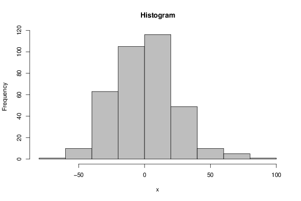
Title produced by software

Histogram

Date of computation

Wed, 12 Dec 2012 09:11:08 -0500

Cite this page as follows

Statistical Computations at FreeStatistics.org, Office for Research Development and Education, URL https://freestatistics.org/blog/index.php?v=date/2012/Dec/12/t1355321481am59imj5c76klps.htm/, Retrieved Mon, 29 Apr 2024 09:56:57 +0000

Statistical Computations at FreeStatistics.org, Office for Research Development and Education, URL https://freestatistics.org/blog/index.php?pk=198890, Retrieved Mon, 29 Apr 2024 09:56:57 +0000

QR Codes:

Paste this QR Code to cite your computation.

Original text written by user:

IsPrivate?

No (this computation is public)

User-defined keywords

Estimated Impact

Family? (F = Feedback message, R = changed R code, M = changed R Module, P = changed Parameters, D = changed Data)

-       [Histogram] [cdhist] [2012-12-12 14:11:08] [e357aba3893873b930815b56a53f1005] [Current]

Feedback Forum

Post a new message

Dataseries X:

Download CSV

Histogram

Boxplots

NA
NA
NA
NA
NA
NA
-6.141574074074070
2.766759259259260
-2.474768518518540
-24.749212962963000
-27.341990740740700
-24.099629629629600
-33.038657407407400
-8.168935185185200
-7.480462962962920
7.314953703703800
37.235092592592600
-3.204907407407350
51.437592592592600
27.533425925925900
4.379398148148080
30.009120370370400
-13.662824074074000
-0.0871296296296009
28.698842592592600
45.426898148148200
31.498703703703800
19.148287037037100
12.155925925925900
-21.496574074074000
-5.812407407407420
-26.724907407407400
-3.037268518518490
-15.228379629629600
6.978842592592570
23.204537037037100
-14.909490740740800
-25.098101851851800
-17.213796296296200
-11.485046296296200
-4.577407407407350
-37.146574074074100
-13.445740740740700
-5.920740740740710
22.550231481481500
26.934120370370400
29.599675925925900
9.358703703703700
-17.288657407407400
-17.243935185185200
-27.347129629629600
-1.689212962962960
16.630925925926000
-28.521574074074100
3.866759259259250
20.929259259259300
22.529398148148100
14.575787037037000
5.991342592592590
2.158703703703710
-9.538657407407440
-30.718935185185200
-18.667962962962900
15.460787037037100
11.443425925925900
-46.979907407407400
-33.029074074074100
-35.524907407407400
-24.133101851851800
-30.890879629629600
-25.216990740740800
-8.687129629629570
21.478009259259300
39.681064814814800
52.869537037037000
61.014953703703700
52.914259259259300
-24.896574074074100
-2.716574074074060
9.329259259259230
28.746064814814800
0.100787037037037
4.274675925925920
-0.216296296296264
0.0946759259259125
-9.410601851851880
-4.651296296296270
29.556620370370400
8.385092592592570
-40.050740740740800
-33.420740740740800
-9.849907407407440
-8.512268518518510
4.634120370370400
9.953842592592600
13.600370370370400
-15.642824074074000
-21.731435185185100
2.632037037037090
5.664953703703760
36.035092592592500
0.678425925925978
5.866759259259250
-14.716574074074100
-14.641435185185200
-15.536712962963000
14.983009259259200
20.758703703703700
2.936342592592670
-16.456435185185100
-20.455462962963000
-2.014212962962920
15.955925925925900
-12.292407407407400
-23.616574074074000
-37.349907407407400
-39.524768518518400
-47.378379629629500
-21.796157407407500
-20.374629629629700
1.503009259259220
41.001898148148300
53.257037037037100
72.781620370370400
62.414259259259400
22.857592592592700
31.916759259259300
15.337592592592600
-15.941435185185200
-21.074212962962900
-26.337824074074000
13.037870370370400
13.061342592592700
18.897731481481500
11.248703703703700
-16.535046296296200
-15.923240740740700
-40.571574074074000
-27.945740740740700
-16.362407407407400
-9.312268518518580
10.463287037037000
29.228842592592600
14.667037037037100
-1.538657407407360
-35.152268518518500
14.136203703703700
-2.880879629629530
-7.306574074074090
-6.288240740740660
-18.591574074074100
-16.654074074074100
-50.558101851851900
-23.115879629629700
-12.137824074074000
26.821203703703700
30.869675925925900
47.610231481481500
41.982037037037000
24.485787037037000
22.564259259259400
15.811759259259200
10.891759259259300
-1.674907407407370
-14.495601851851900
-6.924212962962880
-13.171157407407300
3.175370370370440
-2.759490740740660
-17.185601851851900
-4.576296296296330
-5.085046296296240
28.260092592592500
-15.821574074074000
-28.158240740740700
3.166759259259270
-19.341435185185100
-26.657546296296300
0.703842592592707
1.512870370370360
12.311342592592700
28.043564814814800
9.048703703703780
3.877453703703740
19.189259259259300
6.174259259259320
-9.370740740740640
-14.041574074074100
-21.624768518518500
-11.824212962963000
15.695509259259300
9.662870370370290
11.811342592592600
1.264398148148130
2.886203703703760
5.627453703703800
-0.677407407407429
22.803425925925900
-25.495740740740700
-2.616574074074040
-9.812268518518580
3.213287037037050
-3.375324074074060
7.475370370370340
-9.859490740740630
8.239398148148210
-12.197129629629600
11.348287037037100
8.305925925925920
24.136759259259300
-7.654074074074060
4.950092592592570
-1.658101851851940
6.992453703703750
8.512175925925990
0.99620370370377
-23.096990740740800
-41.218935185185200
-26.767962962962900
-9.880879629629650
19.651759259259200
28.503425925926000
0.687592592592637
9.500092592592580
-4.153935185185160
8.292453703703760
0.0538425925926731
8.692037037037040
-16.096990740740700
-22.564768518518500
-24.197129629629700
-16.401712962962900
-19.452407407407400
23.120092592592600
10.862592592592600
11.758425925925900
25.041898148148100
47.388287037037000
22.541342592592600
3.729537037037060
-33.892824074074100
-19.385601851851800
-29.772129629629600
-30.072546296296300
-24.639907407407400
36.232592592592700
24.037592592592600
13.554259259259300
17.637731481481500
24.304953703703700
9.399675925925980
-6.653796296296260
-33.080324074074100
-36.177268518518500
-32.142962962963000
-15.022546296296300
-20.227407407407400
14.495092592592600
16.129259259259200
10.758425925926000
30.129398148148100
25.834120370370400
-17.200324074074000
-36.553796296296300
-42.726157407407400
-22.718935185185100
-16.497129629629600
-5.610046296296220
-15.298240740740800
24.078425925925900
16.958425925925900
4.395925925925840
17.029398148148100
18.784120370370400
23.308009259259300
17.371203703703800
15.123842592592600
3.368564814814870
-5.613796296296300
-16.835046296296300
-28.069074074074100
7.570092592592570
16.704259259259200
21.462592592592600
17.629398148148100
6.271620370370390
9.658009259259300
-3.074629629629610
-0.163657407407300
-9.793935185185030
-4.380462962962890
-14.547546296296300
-26.214907407407400
13.836759259259400
19.683425925925900
25.333425925926000
29.033564814814800
31.163287037037000
-6.096157407407420
-17.620462962963000
-29.921990740740700
-15.256435185185200
-20.292962962962900
-8.635046296296310
-21.385740740740700
11.682592592592700
6.354259259259320
1.208425925925890
12.975231481481500
-12.945046296296300
-6.921157407407350
-11.587129629629700
5.023842592592640
4.810231481481480
-17.326296296296300
-31.926712962962900
-38.823240740740700
-3.392407407407350
-11.624907407407400
-43.874907407407400
-22.087268518518400
-51.745046296296200
-38.112824074074100
-25.003796296296300
83.611342592592700
64.876898148148300
72.002870370370500
39.727453703703800
25.347592592592700
36.120092592592600
21.125092592592600
2.670925925926210
8.204398148148360
3.575787037037120
-9.662824074074020
-5.166296296296200
25.965509259259300
8.422731481481500
-15.247129629629600
-34.510046296296400
-69.902407407407600
-6.363240740740710
13.433425925926100
20.645925925926100
8.908564814815000
6.642453703703720
13.512175925926000
6.483703703703780
19.365509259259400
42.835231481481600
15.848703703703800
-37.489212962963100
-52.589907407407400
12.640925925925900
-4.320740740740920
18.620925925925900
15.125231481481600
17.500787037037200
15.249675925926000
-24.970462962963000
10.311342592592600
-7.585601851851950
-3.972129629629650
-36.776712962963100
-32.789907407407400
-15.104907407407400
NA
NA
NA
NA
NA
NA

Summary of computational transaction
Raw Input	view raw input (R code)
Raw Output	view raw output of R engine
Computing time	2 seconds
R Server	'Gwilym Jenkins' @ jenkins.wessa.net

\begin{tabular}{lllllllll}
\hline
Summary of computational transaction \tabularnewline
Raw Input & view raw input (R code)  \tabularnewline
Raw Output & view raw output of R engine  \tabularnewline
Computing time & 2 seconds \tabularnewline
R Server & 'Gwilym Jenkins' @ jenkins.wessa.net \tabularnewline
\hline
\end{tabular}
%Source: https://freestatistics.org/blog/index.php?pk=198890&T=0

[TABLE]
[ROW][C]Summary of computational transaction[/C][/ROW]
[ROW][C]Raw Input[/C][C]view raw input (R code) [/C][/ROW]
[ROW][C]Raw Output[/C][C]view raw output of R engine [/C][/ROW]
[ROW][C]Computing time[/C][C]2 seconds[/C][/ROW]
[ROW][C]R Server[/C][C]'Gwilym Jenkins' @ jenkins.wessa.net[/C][/ROW]
[/TABLE]
Source: https://freestatistics.org/blog/index.php?pk=198890&T=0

Globally Unique Identifier (entire table): ba.freestatistics.org/blog/index.php?pk=198890&T=0

As an alternative you can also use a QR Code:

The GUIDs for individual cells are displayed in the table below:

Summary of computational transaction
Raw Input	view raw input (R code)
Raw Output	view raw output of R engine
Computing time	2 seconds
R Server	'Gwilym Jenkins' @ jenkins.wessa.net

Frequency Table (Histogram)
Bins	Midpoint	Abs. Frequency	Rel. Frequency	Cumul. Rel. Freq.	Density
[-80,-60[	-70	1	0.002688	0.002688	0.000139
[-60,-40[	-50	10	0.026882	0.02957	0.001389
[-40,-20[	-30	63	0.169355	0.198925	0.00875
[-20,0[	-10	105	0.282258	0.481183	0.014583
[0,20[	10	116	0.311828	0.793011	0.016111
[20,40[	30	49	0.13172	0.924731	0.006806
[40,60[	50	10	0.026882	0.951613	0.001389
[60,80[	70	5	0.013441	0.965054	0.000694
[80,100]	90	1	0.002688	0.967742	0.000139

\begin{tabular}{lllllllll}
\hline
Frequency Table (Histogram) \tabularnewline
Bins & Midpoint & Abs. Frequency & Rel. Frequency & Cumul. Rel. Freq. & Density \tabularnewline
[-80,-60[ & -70 & 1 & 0.002688 & 0.002688 & 0.000139 \tabularnewline
[-60,-40[ & -50 & 10 & 0.026882 & 0.02957 & 0.001389 \tabularnewline
[-40,-20[ & -30 & 63 & 0.169355 & 0.198925 & 0.00875 \tabularnewline
[-20,0[ & -10 & 105 & 0.282258 & 0.481183 & 0.014583 \tabularnewline
[0,20[ & 10 & 116 & 0.311828 & 0.793011 & 0.016111 \tabularnewline
[20,40[ & 30 & 49 & 0.13172 & 0.924731 & 0.006806 \tabularnewline
[40,60[ & 50 & 10 & 0.026882 & 0.951613 & 0.001389 \tabularnewline
[60,80[ & 70 & 5 & 0.013441 & 0.965054 & 0.000694 \tabularnewline
[80,100] & 90 & 1 & 0.002688 & 0.967742 & 0.000139 \tabularnewline
\hline
\end{tabular}
%Source: https://freestatistics.org/blog/index.php?pk=198890&T=1

[TABLE]
[ROW][C]Frequency Table (Histogram)[/C][/ROW]
[ROW][C]Bins[/C][C]Midpoint[/C][C]Abs. Frequency[/C][C]Rel. Frequency[/C][C]Cumul. Rel. Freq.[/C][C]Density[/C][/ROW]
[ROW][C][-80,-60[[/C][C]-70[/C][C]1[/C][C]0.002688[/C][C]0.002688[/C][C]0.000139[/C][/ROW]
[ROW][C][-60,-40[[/C][C]-50[/C][C]10[/C][C]0.026882[/C][C]0.02957[/C][C]0.001389[/C][/ROW]
[ROW][C][-40,-20[[/C][C]-30[/C][C]63[/C][C]0.169355[/C][C]0.198925[/C][C]0.00875[/C][/ROW]
[ROW][C][-20,0[[/C][C]-10[/C][C]105[/C][C]0.282258[/C][C]0.481183[/C][C]0.014583[/C][/ROW]
[ROW][C][0,20[[/C][C]10[/C][C]116[/C][C]0.311828[/C][C]0.793011[/C][C]0.016111[/C][/ROW]
[ROW][C][20,40[[/C][C]30[/C][C]49[/C][C]0.13172[/C][C]0.924731[/C][C]0.006806[/C][/ROW]
[ROW][C][40,60[[/C][C]50[/C][C]10[/C][C]0.026882[/C][C]0.951613[/C][C]0.001389[/C][/ROW]
[ROW][C][60,80[[/C][C]70[/C][C]5[/C][C]0.013441[/C][C]0.965054[/C][C]0.000694[/C][/ROW]
[ROW][C][80,100][/C][C]90[/C][C]1[/C][C]0.002688[/C][C]0.967742[/C][C]0.000139[/C][/ROW]
[/TABLE]
Source: https://freestatistics.org/blog/index.php?pk=198890&T=1

Globally Unique Identifier (entire table): ba.freestatistics.org/blog/index.php?pk=198890&T=1

As an alternative you can also use a QR Code:

The GUIDs for individual cells are displayed in the table below:

Frequency Table (Histogram)
Bins	Midpoint	Abs. Frequency	Rel. Frequency	Cumul. Rel. Freq.	Density
[-80,-60[	-70	1	0.002688	0.002688	0.000139
[-60,-40[	-50	10	0.026882	0.02957	0.001389
[-40,-20[	-30	63	0.169355	0.198925	0.00875
[-20,0[	-10	105	0.282258	0.481183	0.014583
[0,20[	10	116	0.311828	0.793011	0.016111
[20,40[	30	49	0.13172	0.924731	0.006806
[40,60[	50	10	0.026882	0.951613	0.001389
[60,80[	70	5	0.013441	0.965054	0.000694
[80,100]	90	1	0.002688	0.967742	0.000139

Figure 1

PNG link

Postscript link

PDF link

Parameters (Session):

par2 = grey ; par3 = FALSE ; par4 = Unknown ;

Parameters (R input):

par1 = ; par2 = grey ; par3 = FALSE ; par4 = Unknown ;

R code (references can be found in the software module):

par1 <- as.numeric(par1)
if (par3 == 'TRUE') par3 <- TRUE
if (par3 == 'FALSE') par3 <- FALSE
if (par4 == 'Unknown') par1 <- as.numeric(par1)
if (par4 == 'Interval/Ratio') par1 <- as.numeric(par1)
if (par4 == '3-point Likert') par1 <- c(1:3 - 0.5, 3.5)
if (par4 == '4-point Likert') par1 <- c(1:4 - 0.5, 4.5)
if (par4 == '5-point Likert') par1 <- c(1:5 - 0.5, 5.5)
if (par4 == '6-point Likert') par1 <- c(1:6 - 0.5, 6.5)
if (par4 == '7-point Likert') par1 <- c(1:7 - 0.5, 7.5)
if (par4 == '8-point Likert') par1 <- c(1:8 - 0.5, 8.5)
if (par4 == '9-point Likert') par1 <- c(1:9 - 0.5, 9.5)
if (par4 == '10-point Likert') par1 <- c(1:10 - 0.5, 10.5)
bitmap(file='test1.png')
if(is.numeric(x[1])) {
if (is.na(par1)) {
myhist<-hist(x,col=par2,main=main,xlab=xlab,right=par3)
} else {
if (par1 < 0) par1 <- 3
if (par1 > 50) par1 <- 50
myhist<-hist(x,breaks=par1,col=par2,main=main,xlab=xlab,right=par3)
}
} else {
plot(mytab <- table(x),col=par2,main='Frequency Plot',xlab=xlab,ylab='Absolute Frequency')
}
dev.off()
if(is.numeric(x[1])) {
myhist
n <- length(x)
load(file='createtable')
a<-table.start()
a<-table.row.start(a)
a<-table.element(a,hyperlink('histogram.htm','Frequency Table (Histogram)',''),6,TRUE)
a<-table.row.end(a)
a<-table.row.start(a)
a<-table.element(a,'Bins',header=TRUE)
a<-table.element(a,'Midpoint',header=TRUE)
a<-table.element(a,'Abs. Frequency',header=TRUE)
a<-table.element(a,'Rel. Frequency',header=TRUE)
a<-table.element(a,'Cumul. Rel. Freq.',header=TRUE)
a<-table.element(a,'Density',header=TRUE)
a<-table.row.end(a)
crf <- 0
if (par3 == FALSE) mybracket <- '[' else mybracket <- ']'
mynumrows <- (length(myhist$breaks)-1)
for (i in 1:mynumrows) {
a<-table.row.start(a)
if (i == 1)
dum <- paste('[',myhist$breaks[i],sep='')
else
dum <- paste(mybracket,myhist$breaks[i],sep='')
dum <- paste(dum,myhist$breaks[i+1],sep=',')
if (i==mynumrows)
dum <- paste(dum,']',sep='')
else
dum <- paste(dum,mybracket,sep='')
a<-table.element(a,dum,header=TRUE)
a<-table.element(a,myhist$mids[i])
a<-table.element(a,myhist$counts[i])
rf <- myhist$counts[i]/n
crf <- crf + rf
a<-table.element(a,round(rf,6))
a<-table.element(a,round(crf,6))
a<-table.element(a,round(myhist$density[i],6))
a<-table.row.end(a)
}
a<-table.end(a)
table.save(a,file='mytable.tab')
} else {
mytab
reltab <- mytab / sum(mytab)
n <- length(mytab)
load(file='createtable')
a<-table.start()
a<-table.row.start(a)
a<-table.element(a,'Frequency Table (Categorical Data)',3,TRUE)
a<-table.row.end(a)
a<-table.row.start(a)
a<-table.element(a,'Category',header=TRUE)
a<-table.element(a,'Abs. Frequency',header=TRUE)
a<-table.element(a,'Rel. Frequency',header=TRUE)
a<-table.row.end(a)
for (i in 1:n) {
a<-table.row.start(a)
a<-table.element(a,labels(mytab)$x[i],header=TRUE)
a<-table.element(a,mytab[i])
a<-table.element(a,round(reltab[i],4))
a<-table.row.end(a)
}
a<-table.end(a)
table.save(a,file='mytable1.tab')
}

Free Statistics

Description of Statistical Computation

Tree of Dependent Computations

Dataset

Tables (Output of Computation)

Figures (Output of Computation)

Input Parameters & R Code