Repository of Reproducible Computations

Free Statistics

of Irreproducible Research!

Author's title

Author

*The author of this computation has been verified*

R Software Module

rwasp_regression_trees1.wasp

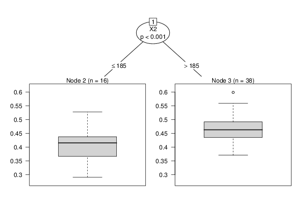
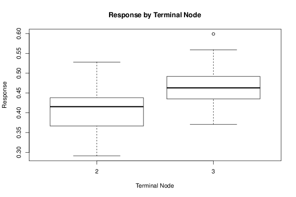
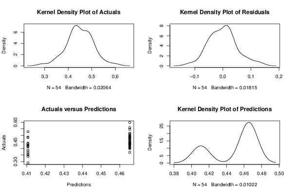
Title produced by software

Recursive Partitioning (Regression Trees)

Date of computation

Tue, 11 Dec 2012 16:03:34 -0500

Cite this page as follows

Statistical Computations at FreeStatistics.org, Office for Research Development and Education, URL https://freestatistics.org/blog/index.php?v=date/2012/Dec/11/t1355259830mbiwand5q22unq7.htm/, Retrieved Thu, 25 Apr 2024 15:22:36 +0000

Statistical Computations at FreeStatistics.org, Office for Research Development and Education, URL https://freestatistics.org/blog/index.php?pk=198704, Retrieved Thu, 25 Apr 2024 15:22:36 +0000

QR Codes:

Paste this QR Code to cite your computation.

Original text written by user:

IsPrivate?

No (this computation is public)

User-defined keywords

Estimated Impact

Family? (F = Feedback message, R = changed R code, M = changed R Module, P = changed Parameters, D = changed Data)

-     [Recursive Partitioning (Regression Trees)] [] [2010-12-05 18:59:57] [b98453cac15ba1066b407e146608df68]
- R PD  [Recursive Partitioning (Regression Trees)] [WS10.4] [2012-12-11 20:38:27] [516331a1326ffbbf54349d9c9d5f2d94]
-   PD    [Recursive Partitioning (Regression Trees)] [WS10.5] [2012-12-11 20:51:39] [516331a1326ffbbf54349d9c9d5f2d94]
-   P       [Recursive Partitioning (Regression Trees)] [WS10.6] [2012-12-11 20:58:50] [516331a1326ffbbf54349d9c9d5f2d94]
-   P           [Recursive Partitioning (Regression Trees)] [WS10.6] [2012-12-11 21:03:34] [6144fd9dab7e8876ce9100c6a2ac91c2] [Current]
-                 [Recursive Partitioning (Regression Trees)] [WS10.7] [2012-12-11 21:06:19] [516331a1326ffbbf54349d9c9d5f2d94] 

Feedback Forum

Post a new message

Dataseries X:

Download CSV

Histogram

Boxplots

6.8	225	0.442	0.672	9.2
6.3	180	0.435	0.797	11.7
6.4	190	0.456	0.761	15.8
6.2	180	0.416	0.651	8.6
6.9	205	0.449	0.9	23.2
6.4	225	0.431	0.78	27.4
6.3	185	0.487	0.771	9.3
6.8	235	0.469	0.75	16
6.9	235	0.435	0.818	4.7
6.7	210	0.48	0.825	12.5
6.9	245	0.516	0.632	20.1
6.9	245	0.493	0.757	9.1
6.3	185	0.374	0.709	8.1
6.1	185	0.424	0.782	8.6
6.2	180	0.441	0.775	20.3
6.8	220	0.503	0.88	25
6.5	194	0.503	0.833	19.2
7.6	225	0.425	0.571	3.3
6.3	210	0.371	0.816	11.2
7.1	240	0.504	0.714	10.5
6.8	225	0.4	0.765	10.1
7.3	263	0.482	0.655	7.2
6.4	210	0.475	0.244	13.6
6.8	235	0.428	0.728	9
7.2	230	0.559	0.721	24.6
6.4	190	0.441	0.757	12.6
6.6	220	0.492	0.747	5.6
6.8	210	0.402	0.739	8.7
6.1	180	0.415	0.713	7.7
6.5	235	0.492	0.742	24.1
6.4	185	0.484	0.861	11.7
6	175	0.387	0.721	7.7
6	192	0.436	0.785	9.6
7.3	263	0.482	0.655	7.2
6.1	180	0.34	0.821	12.3
6.7	240	0.516	0.728	8.9
6.4	210	0.475	0.846	13.6
5.8	160	0.412	0.813	11.2
6.9	230	0.411	0.595	2.8
7	245	0.407	0.573	3.2
7.3	228	0.445	0.726	9.4
5.9	155	0.291	0.707	11.9
6.2	200	0.449	0.804	15.4
6.8	235	0.546	0.784	7.4
7	235	0.48	0.744	18.9
5.9	105	0.359	0.839	7.9
6.1	180	0.528	0.79	12.2
5.7	185	0.352	0.701	11
7.1	245	0.414	0.778	2.8
5.8	180	0.425	0.872	11.8
7.4	240	0.599	0.713	17.1
6.8	225	0.482	0.701	11.6
6.8	215	0.457	0.734	5.8
7	230	0.435	0.764	8.3

Summary of computational transaction
Raw Input	view raw input (R code)
Raw Output	view raw output of R engine
Computing time	4 seconds
R Server	'Gertrude Mary Cox' @ cox.wessa.net

\begin{tabular}{lllllllll}
\hline
Summary of computational transaction \tabularnewline
Raw Input & view raw input (R code)  \tabularnewline
Raw Output & view raw output of R engine  \tabularnewline
Computing time & 4 seconds \tabularnewline
R Server & 'Gertrude Mary Cox' @ cox.wessa.net \tabularnewline
\hline
\end{tabular}
%Source: https://freestatistics.org/blog/index.php?pk=198704&T=0

[TABLE]
[ROW][C]Summary of computational transaction[/C][/ROW]
[ROW][C]Raw Input[/C][C]view raw input (R code) [/C][/ROW]
[ROW][C]Raw Output[/C][C]view raw output of R engine [/C][/ROW]
[ROW][C]Computing time[/C][C]4 seconds[/C][/ROW]
[ROW][C]R Server[/C][C]'Gertrude Mary Cox' @ cox.wessa.net[/C][/ROW]
[/TABLE]
Source: https://freestatistics.org/blog/index.php?pk=198704&T=0

Globally Unique Identifier (entire table): ba.freestatistics.org/blog/index.php?pk=198704&T=0

As an alternative you can also use a QR Code:

The GUIDs for individual cells are displayed in the table below:

Summary of computational transaction
Raw Input	view raw input (R code)
Raw Output	view raw output of R engine
Computing time	4 seconds
R Server	'Gertrude Mary Cox' @ cox.wessa.net

Goodness of Fit
Correlation	0.4457
R-squared	0.1987
RMSE	0.0502

\begin{tabular}{lllllllll}
\hline
Goodness of Fit \tabularnewline
Correlation & 0.4457 \tabularnewline
R-squared & 0.1987 \tabularnewline
RMSE & 0.0502 \tabularnewline
\hline
\end{tabular}
%Source: https://freestatistics.org/blog/index.php?pk=198704&T=1

[TABLE]
[ROW][C]Goodness of Fit[/C][/ROW]
[ROW][C]Correlation[/C][C]0.4457[/C][/ROW]
[ROW][C]R-squared[/C][C]0.1987[/C][/ROW]
[ROW][C]RMSE[/C][C]0.0502[/C][/ROW]
[/TABLE]
Source: https://freestatistics.org/blog/index.php?pk=198704&T=1

Globally Unique Identifier (entire table): ba.freestatistics.org/blog/index.php?pk=198704&T=1

As an alternative you can also use a QR Code:

The GUIDs for individual cells are displayed in the table below:

Goodness of Fit
Correlation	0.4457
R-squared	0.1987
RMSE	0.0502

Actuals, Predictions, and Residuals
#	Actuals	Forecasts	Residuals
1	0.442	0.465315789473684	-0.0233157894736842
2	0.435	0.410625	0.024375
3	0.456	0.465315789473684	-0.00931578947368417
4	0.416	0.410625	0.00537499999999996
5	0.449	0.465315789473684	-0.0163157894736842
6	0.431	0.465315789473684	-0.0343157894736842
7	0.487	0.410625	0.076375
8	0.469	0.465315789473684	0.00368421052631579
9	0.435	0.465315789473684	-0.0303157894736842
10	0.48	0.465315789473684	0.0146842105263158
11	0.516	0.465315789473684	0.0506842105263158
12	0.493	0.465315789473684	0.0276842105263158
13	0.374	0.410625	-0.036625
14	0.424	0.410625	0.013375
15	0.441	0.410625	0.030375
16	0.503	0.465315789473684	0.0376842105263158
17	0.503	0.465315789473684	0.0376842105263158
18	0.425	0.465315789473684	-0.0403157894736842
19	0.371	0.465315789473684	-0.0943157894736842
20	0.504	0.465315789473684	0.0386842105263158
21	0.4	0.465315789473684	-0.0653157894736842
22	0.482	0.465315789473684	0.0166842105263158
23	0.475	0.465315789473684	0.0096842105263158
24	0.428	0.465315789473684	-0.0373157894736842
25	0.559	0.465315789473684	0.0936842105263159
26	0.441	0.465315789473684	-0.0243157894736842
27	0.492	0.465315789473684	0.0266842105263158
28	0.402	0.465315789473684	-0.0633157894736842
29	0.415	0.410625	0.00437499999999996
30	0.492	0.465315789473684	0.0266842105263158
31	0.484	0.410625	0.073375
32	0.387	0.410625	-0.023625
33	0.436	0.465315789473684	-0.0293157894736842
34	0.482	0.465315789473684	0.0166842105263158
35	0.34	0.410625	-0.070625
36	0.516	0.465315789473684	0.0506842105263158
37	0.475	0.465315789473684	0.0096842105263158
38	0.412	0.410625	0.00137499999999996
39	0.411	0.465315789473684	-0.0543157894736842
40	0.407	0.465315789473684	-0.0583157894736842
41	0.445	0.465315789473684	-0.0203157894736842
42	0.291	0.410625	-0.119625
43	0.449	0.465315789473684	-0.0163157894736842
44	0.546	0.465315789473684	0.0806842105263159
45	0.48	0.465315789473684	0.0146842105263158
46	0.359	0.410625	-0.051625
47	0.528	0.410625	0.117375
48	0.352	0.410625	-0.058625
49	0.414	0.465315789473684	-0.0513157894736842
50	0.425	0.410625	0.014375
51	0.599	0.465315789473684	0.133684210526316
52	0.482	0.465315789473684	0.0166842105263158
53	0.457	0.465315789473684	-0.00831578947368417
54	0.435	0.465315789473684	-0.0303157894736842

\begin{tabular}{lllllllll}
\hline
Actuals, Predictions, and Residuals \tabularnewline
# & Actuals & Forecasts & Residuals \tabularnewline
1 & 0.442 & 0.465315789473684 & -0.0233157894736842 \tabularnewline
2 & 0.435 & 0.410625 & 0.024375 \tabularnewline
3 & 0.456 & 0.465315789473684 & -0.00931578947368417 \tabularnewline
4 & 0.416 & 0.410625 & 0.00537499999999996 \tabularnewline
5 & 0.449 & 0.465315789473684 & -0.0163157894736842 \tabularnewline
6 & 0.431 & 0.465315789473684 & -0.0343157894736842 \tabularnewline
7 & 0.487 & 0.410625 & 0.076375 \tabularnewline
8 & 0.469 & 0.465315789473684 & 0.00368421052631579 \tabularnewline
9 & 0.435 & 0.465315789473684 & -0.0303157894736842 \tabularnewline
10 & 0.48 & 0.465315789473684 & 0.0146842105263158 \tabularnewline
11 & 0.516 & 0.465315789473684 & 0.0506842105263158 \tabularnewline
12 & 0.493 & 0.465315789473684 & 0.0276842105263158 \tabularnewline
13 & 0.374 & 0.410625 & -0.036625 \tabularnewline
14 & 0.424 & 0.410625 & 0.013375 \tabularnewline
15 & 0.441 & 0.410625 & 0.030375 \tabularnewline
16 & 0.503 & 0.465315789473684 & 0.0376842105263158 \tabularnewline
17 & 0.503 & 0.465315789473684 & 0.0376842105263158 \tabularnewline
18 & 0.425 & 0.465315789473684 & -0.0403157894736842 \tabularnewline
19 & 0.371 & 0.465315789473684 & -0.0943157894736842 \tabularnewline
20 & 0.504 & 0.465315789473684 & 0.0386842105263158 \tabularnewline
21 & 0.4 & 0.465315789473684 & -0.0653157894736842 \tabularnewline
22 & 0.482 & 0.465315789473684 & 0.0166842105263158 \tabularnewline
23 & 0.475 & 0.465315789473684 & 0.0096842105263158 \tabularnewline
24 & 0.428 & 0.465315789473684 & -0.0373157894736842 \tabularnewline
25 & 0.559 & 0.465315789473684 & 0.0936842105263159 \tabularnewline
26 & 0.441 & 0.465315789473684 & -0.0243157894736842 \tabularnewline
27 & 0.492 & 0.465315789473684 & 0.0266842105263158 \tabularnewline
28 & 0.402 & 0.465315789473684 & -0.0633157894736842 \tabularnewline
29 & 0.415 & 0.410625 & 0.00437499999999996 \tabularnewline
30 & 0.492 & 0.465315789473684 & 0.0266842105263158 \tabularnewline
31 & 0.484 & 0.410625 & 0.073375 \tabularnewline
32 & 0.387 & 0.410625 & -0.023625 \tabularnewline
33 & 0.436 & 0.465315789473684 & -0.0293157894736842 \tabularnewline
34 & 0.482 & 0.465315789473684 & 0.0166842105263158 \tabularnewline
35 & 0.34 & 0.410625 & -0.070625 \tabularnewline
36 & 0.516 & 0.465315789473684 & 0.0506842105263158 \tabularnewline
37 & 0.475 & 0.465315789473684 & 0.0096842105263158 \tabularnewline
38 & 0.412 & 0.410625 & 0.00137499999999996 \tabularnewline
39 & 0.411 & 0.465315789473684 & -0.0543157894736842 \tabularnewline
40 & 0.407 & 0.465315789473684 & -0.0583157894736842 \tabularnewline
41 & 0.445 & 0.465315789473684 & -0.0203157894736842 \tabularnewline
42 & 0.291 & 0.410625 & -0.119625 \tabularnewline
43 & 0.449 & 0.465315789473684 & -0.0163157894736842 \tabularnewline
44 & 0.546 & 0.465315789473684 & 0.0806842105263159 \tabularnewline
45 & 0.48 & 0.465315789473684 & 0.0146842105263158 \tabularnewline
46 & 0.359 & 0.410625 & -0.051625 \tabularnewline
47 & 0.528 & 0.410625 & 0.117375 \tabularnewline
48 & 0.352 & 0.410625 & -0.058625 \tabularnewline
49 & 0.414 & 0.465315789473684 & -0.0513157894736842 \tabularnewline
50 & 0.425 & 0.410625 & 0.014375 \tabularnewline
51 & 0.599 & 0.465315789473684 & 0.133684210526316 \tabularnewline
52 & 0.482 & 0.465315789473684 & 0.0166842105263158 \tabularnewline
53 & 0.457 & 0.465315789473684 & -0.00831578947368417 \tabularnewline
54 & 0.435 & 0.465315789473684 & -0.0303157894736842 \tabularnewline
\hline
\end{tabular}
%Source: https://freestatistics.org/blog/index.php?pk=198704&T=2

[TABLE]
[ROW][C]Actuals, Predictions, and Residuals[/C][/ROW]
[ROW][C]#[/C][C]Actuals[/C][C]Forecasts[/C][C]Residuals[/C][/ROW]
[ROW][C]1[/C][C]0.442[/C][C]0.465315789473684[/C][C]-0.0233157894736842[/C][/ROW]
[ROW][C]2[/C][C]0.435[/C][C]0.410625[/C][C]0.024375[/C][/ROW]
[ROW][C]3[/C][C]0.456[/C][C]0.465315789473684[/C][C]-0.00931578947368417[/C][/ROW]
[ROW][C]4[/C][C]0.416[/C][C]0.410625[/C][C]0.00537499999999996[/C][/ROW]
[ROW][C]5[/C][C]0.449[/C][C]0.465315789473684[/C][C]-0.0163157894736842[/C][/ROW]
[ROW][C]6[/C][C]0.431[/C][C]0.465315789473684[/C][C]-0.0343157894736842[/C][/ROW]
[ROW][C]7[/C][C]0.487[/C][C]0.410625[/C][C]0.076375[/C][/ROW]
[ROW][C]8[/C][C]0.469[/C][C]0.465315789473684[/C][C]0.00368421052631579[/C][/ROW]
[ROW][C]9[/C][C]0.435[/C][C]0.465315789473684[/C][C]-0.0303157894736842[/C][/ROW]
[ROW][C]10[/C][C]0.48[/C][C]0.465315789473684[/C][C]0.0146842105263158[/C][/ROW]
[ROW][C]11[/C][C]0.516[/C][C]0.465315789473684[/C][C]0.0506842105263158[/C][/ROW]
[ROW][C]12[/C][C]0.493[/C][C]0.465315789473684[/C][C]0.0276842105263158[/C][/ROW]
[ROW][C]13[/C][C]0.374[/C][C]0.410625[/C][C]-0.036625[/C][/ROW]
[ROW][C]14[/C][C]0.424[/C][C]0.410625[/C][C]0.013375[/C][/ROW]
[ROW][C]15[/C][C]0.441[/C][C]0.410625[/C][C]0.030375[/C][/ROW]
[ROW][C]16[/C][C]0.503[/C][C]0.465315789473684[/C][C]0.0376842105263158[/C][/ROW]
[ROW][C]17[/C][C]0.503[/C][C]0.465315789473684[/C][C]0.0376842105263158[/C][/ROW]
[ROW][C]18[/C][C]0.425[/C][C]0.465315789473684[/C][C]-0.0403157894736842[/C][/ROW]
[ROW][C]19[/C][C]0.371[/C][C]0.465315789473684[/C][C]-0.0943157894736842[/C][/ROW]
[ROW][C]20[/C][C]0.504[/C][C]0.465315789473684[/C][C]0.0386842105263158[/C][/ROW]
[ROW][C]21[/C][C]0.4[/C][C]0.465315789473684[/C][C]-0.0653157894736842[/C][/ROW]
[ROW][C]22[/C][C]0.482[/C][C]0.465315789473684[/C][C]0.0166842105263158[/C][/ROW]
[ROW][C]23[/C][C]0.475[/C][C]0.465315789473684[/C][C]0.0096842105263158[/C][/ROW]
[ROW][C]24[/C][C]0.428[/C][C]0.465315789473684[/C][C]-0.0373157894736842[/C][/ROW]
[ROW][C]25[/C][C]0.559[/C][C]0.465315789473684[/C][C]0.0936842105263159[/C][/ROW]
[ROW][C]26[/C][C]0.441[/C][C]0.465315789473684[/C][C]-0.0243157894736842[/C][/ROW]
[ROW][C]27[/C][C]0.492[/C][C]0.465315789473684[/C][C]0.0266842105263158[/C][/ROW]
[ROW][C]28[/C][C]0.402[/C][C]0.465315789473684[/C][C]-0.0633157894736842[/C][/ROW]
[ROW][C]29[/C][C]0.415[/C][C]0.410625[/C][C]0.00437499999999996[/C][/ROW]
[ROW][C]30[/C][C]0.492[/C][C]0.465315789473684[/C][C]0.0266842105263158[/C][/ROW]
[ROW][C]31[/C][C]0.484[/C][C]0.410625[/C][C]0.073375[/C][/ROW]
[ROW][C]32[/C][C]0.387[/C][C]0.410625[/C][C]-0.023625[/C][/ROW]
[ROW][C]33[/C][C]0.436[/C][C]0.465315789473684[/C][C]-0.0293157894736842[/C][/ROW]
[ROW][C]34[/C][C]0.482[/C][C]0.465315789473684[/C][C]0.0166842105263158[/C][/ROW]
[ROW][C]35[/C][C]0.34[/C][C]0.410625[/C][C]-0.070625[/C][/ROW]
[ROW][C]36[/C][C]0.516[/C][C]0.465315789473684[/C][C]0.0506842105263158[/C][/ROW]
[ROW][C]37[/C][C]0.475[/C][C]0.465315789473684[/C][C]0.0096842105263158[/C][/ROW]
[ROW][C]38[/C][C]0.412[/C][C]0.410625[/C][C]0.00137499999999996[/C][/ROW]
[ROW][C]39[/C][C]0.411[/C][C]0.465315789473684[/C][C]-0.0543157894736842[/C][/ROW]
[ROW][C]40[/C][C]0.407[/C][C]0.465315789473684[/C][C]-0.0583157894736842[/C][/ROW]
[ROW][C]41[/C][C]0.445[/C][C]0.465315789473684[/C][C]-0.0203157894736842[/C][/ROW]
[ROW][C]42[/C][C]0.291[/C][C]0.410625[/C][C]-0.119625[/C][/ROW]
[ROW][C]43[/C][C]0.449[/C][C]0.465315789473684[/C][C]-0.0163157894736842[/C][/ROW]
[ROW][C]44[/C][C]0.546[/C][C]0.465315789473684[/C][C]0.0806842105263159[/C][/ROW]
[ROW][C]45[/C][C]0.48[/C][C]0.465315789473684[/C][C]0.0146842105263158[/C][/ROW]
[ROW][C]46[/C][C]0.359[/C][C]0.410625[/C][C]-0.051625[/C][/ROW]
[ROW][C]47[/C][C]0.528[/C][C]0.410625[/C][C]0.117375[/C][/ROW]
[ROW][C]48[/C][C]0.352[/C][C]0.410625[/C][C]-0.058625[/C][/ROW]
[ROW][C]49[/C][C]0.414[/C][C]0.465315789473684[/C][C]-0.0513157894736842[/C][/ROW]
[ROW][C]50[/C][C]0.425[/C][C]0.410625[/C][C]0.014375[/C][/ROW]
[ROW][C]51[/C][C]0.599[/C][C]0.465315789473684[/C][C]0.133684210526316[/C][/ROW]
[ROW][C]52[/C][C]0.482[/C][C]0.465315789473684[/C][C]0.0166842105263158[/C][/ROW]
[ROW][C]53[/C][C]0.457[/C][C]0.465315789473684[/C][C]-0.00831578947368417[/C][/ROW]
[ROW][C]54[/C][C]0.435[/C][C]0.465315789473684[/C][C]-0.0303157894736842[/C][/ROW]
[/TABLE]
Source: https://freestatistics.org/blog/index.php?pk=198704&T=2

Globally Unique Identifier (entire table): ba.freestatistics.org/blog/index.php?pk=198704&T=2

As an alternative you can also use a QR Code:

The GUIDs for individual cells are displayed in the table below:

Actuals, Predictions, and Residuals
#	Actuals	Forecasts	Residuals
1	0.442	0.465315789473684	-0.0233157894736842
2	0.435	0.410625	0.024375
3	0.456	0.465315789473684	-0.00931578947368417
4	0.416	0.410625	0.00537499999999996
5	0.449	0.465315789473684	-0.0163157894736842
6	0.431	0.465315789473684	-0.0343157894736842
7	0.487	0.410625	0.076375
8	0.469	0.465315789473684	0.00368421052631579
9	0.435	0.465315789473684	-0.0303157894736842
10	0.48	0.465315789473684	0.0146842105263158
11	0.516	0.465315789473684	0.0506842105263158
12	0.493	0.465315789473684	0.0276842105263158
13	0.374	0.410625	-0.036625
14	0.424	0.410625	0.013375
15	0.441	0.410625	0.030375
16	0.503	0.465315789473684	0.0376842105263158
17	0.503	0.465315789473684	0.0376842105263158
18	0.425	0.465315789473684	-0.0403157894736842
19	0.371	0.465315789473684	-0.0943157894736842
20	0.504	0.465315789473684	0.0386842105263158
21	0.4	0.465315789473684	-0.0653157894736842
22	0.482	0.465315789473684	0.0166842105263158
23	0.475	0.465315789473684	0.0096842105263158
24	0.428	0.465315789473684	-0.0373157894736842
25	0.559	0.465315789473684	0.0936842105263159
26	0.441	0.465315789473684	-0.0243157894736842
27	0.492	0.465315789473684	0.0266842105263158
28	0.402	0.465315789473684	-0.0633157894736842
29	0.415	0.410625	0.00437499999999996
30	0.492	0.465315789473684	0.0266842105263158
31	0.484	0.410625	0.073375
32	0.387	0.410625	-0.023625
33	0.436	0.465315789473684	-0.0293157894736842
34	0.482	0.465315789473684	0.0166842105263158
35	0.34	0.410625	-0.070625
36	0.516	0.465315789473684	0.0506842105263158
37	0.475	0.465315789473684	0.0096842105263158
38	0.412	0.410625	0.00137499999999996
39	0.411	0.465315789473684	-0.0543157894736842
40	0.407	0.465315789473684	-0.0583157894736842
41	0.445	0.465315789473684	-0.0203157894736842
42	0.291	0.410625	-0.119625
43	0.449	0.465315789473684	-0.0163157894736842
44	0.546	0.465315789473684	0.0806842105263159
45	0.48	0.465315789473684	0.0146842105263158
46	0.359	0.410625	-0.051625
47	0.528	0.410625	0.117375
48	0.352	0.410625	-0.058625
49	0.414	0.465315789473684	-0.0513157894736842
50	0.425	0.410625	0.014375
51	0.599	0.465315789473684	0.133684210526316
52	0.482	0.465315789473684	0.0166842105263158
53	0.457	0.465315789473684	-0.00831578947368417
54	0.435	0.465315789473684	-0.0303157894736842

Figure 1

PNG link

Postscript link

PDF link

Figure 2

PNG link

Postscript link

PDF link

Figure 3

PNG link

Postscript link

PDF link

Parameters (Session):

par1 = 3 ; par2 = none ; par3 = 4 ; par4 = no ;

Parameters (R input):

par1 = 3 ; par2 = none ; par3 = 4 ; par4 = no ;

R code (references can be found in the software module):

library(party)
library(Hmisc)
par1 <- as.numeric(par1)
par3 <- as.numeric(par3)
x <- data.frame(t(y))
is.data.frame(x)
x <- x[!is.na(x[,par1]),]
k <- length(x[1,])
n <- length(x[,1])
colnames(x)[par1]
x[,par1]
if (par2 == 'kmeans') {
cl <- kmeans(x[,par1], par3)
print(cl)
clm <- matrix(cbind(cl$centers,1:par3),ncol=2)
clm <- clm[sort.list(clm[,1]),]
for (i in 1:par3) {
cl$cluster[cl$cluster==clm[i,2]] <- paste('C',i,sep='')
}
cl$cluster <- as.factor(cl$cluster)
print(cl$cluster)
x[,par1] <- cl$cluster
}
if (par2 == 'quantiles') {
x[,par1] <- cut2(x[,par1],g=par3)
}
if (par2 == 'hclust') {
hc <- hclust(dist(x[,par1])^2, 'cen')
print(hc)
memb <- cutree(hc, k = par3)
dum <- c(mean(x[memb==1,par1]))
for (i in 2:par3) {
dum <- c(dum, mean(x[memb==i,par1]))
}
hcm <- matrix(cbind(dum,1:par3),ncol=2)
hcm <- hcm[sort.list(hcm[,1]),]
for (i in 1:par3) {
memb[memb==hcm[i,2]] <- paste('C',i,sep='')
}
memb <- as.factor(memb)
print(memb)
x[,par1] <- memb
}
if (par2=='equal') {
ed <- cut(as.numeric(x[,par1]),par3,labels=paste('C',1:par3,sep=''))
x[,par1] <- as.factor(ed)
}
table(x[,par1])
colnames(x)
colnames(x)[par1]
x[,par1]
if (par2 == 'none') {
m <- ctree(as.formula(paste(colnames(x)[par1],' ~ .',sep='')),data = x)
}
load(file='createtable')
if (par2 != 'none') {
m <- ctree(as.formula(paste('as.factor(',colnames(x)[par1],') ~ .',sep='')),data = x)
if (par4=='yes') {
a<-table.start()
a<-table.row.start(a)
a<-table.element(a,'10-Fold Cross Validation',3+2*par3,TRUE)
a<-table.row.end(a)
a<-table.row.start(a)
a<-table.element(a,'',1,TRUE)
a<-table.element(a,'Prediction (training)',par3+1,TRUE)
a<-table.element(a,'Prediction (testing)',par3+1,TRUE)
a<-table.row.end(a)
a<-table.row.start(a)
a<-table.element(a,'Actual',1,TRUE)
for (jjj in 1:par3) a<-table.element(a,paste('C',jjj,sep=''),1,TRUE)
a<-table.element(a,'CV',1,TRUE)
for (jjj in 1:par3) a<-table.element(a,paste('C',jjj,sep=''),1,TRUE)
a<-table.element(a,'CV',1,TRUE)
a<-table.row.end(a)
for (i in 1:10) {
ind <- sample(2, nrow(x), replace=T, prob=c(0.9,0.1))
m.ct <- ctree(as.formula(paste('as.factor(',colnames(x)[par1],') ~ .',sep='')),data =x[ind==1,])
if (i==1) {
m.ct.i.pred <- predict(m.ct, newdata=x[ind==1,])
m.ct.i.actu <- x[ind==1,par1]
m.ct.x.pred <- predict(m.ct, newdata=x[ind==2,])
m.ct.x.actu <- x[ind==2,par1]
} else {
m.ct.i.pred <- c(m.ct.i.pred,predict(m.ct, newdata=x[ind==1,]))
m.ct.i.actu <- c(m.ct.i.actu,x[ind==1,par1])
m.ct.x.pred <- c(m.ct.x.pred,predict(m.ct, newdata=x[ind==2,]))
m.ct.x.actu <- c(m.ct.x.actu,x[ind==2,par1])
}
}
print(m.ct.i.tab <- table(m.ct.i.actu,m.ct.i.pred))
numer <- 0
for (i in 1:par3) {
print(m.ct.i.tab[i,i] / sum(m.ct.i.tab[i,]))
numer <- numer + m.ct.i.tab[i,i]
}
print(m.ct.i.cp <- numer / sum(m.ct.i.tab))
print(m.ct.x.tab <- table(m.ct.x.actu,m.ct.x.pred))
numer <- 0
for (i in 1:par3) {
print(m.ct.x.tab[i,i] / sum(m.ct.x.tab[i,]))
numer <- numer + m.ct.x.tab[i,i]
}
print(m.ct.x.cp <- numer / sum(m.ct.x.tab))
for (i in 1:par3) {
a<-table.row.start(a)
a<-table.element(a,paste('C',i,sep=''),1,TRUE)
for (jjj in 1:par3) a<-table.element(a,m.ct.i.tab[i,jjj])
a<-table.element(a,round(m.ct.i.tab[i,i]/sum(m.ct.i.tab[i,]),4))
for (jjj in 1:par3) a<-table.element(a,m.ct.x.tab[i,jjj])
a<-table.element(a,round(m.ct.x.tab[i,i]/sum(m.ct.x.tab[i,]),4))
a<-table.row.end(a)
}
a<-table.row.start(a)
a<-table.element(a,'Overall',1,TRUE)
for (jjj in 1:par3) a<-table.element(a,'-')
a<-table.element(a,round(m.ct.i.cp,4))
for (jjj in 1:par3) a<-table.element(a,'-')
a<-table.element(a,round(m.ct.x.cp,4))
a<-table.row.end(a)
a<-table.end(a)
table.save(a,file='mytable3.tab')
}
}
m
bitmap(file='test1.png')
plot(m)
dev.off()
bitmap(file='test1a.png')
plot(x[,par1] ~ as.factor(where(m)),main='Response by Terminal Node',xlab='Terminal Node',ylab='Response')
dev.off()
if (par2 == 'none') {
forec <- predict(m)
result <- as.data.frame(cbind(x[,par1],forec,x[,par1]-forec))
colnames(result) <- c('Actuals','Forecasts','Residuals')
print(result)
}
if (par2 != 'none') {
print(cbind(as.factor(x[,par1]),predict(m)))
myt <- table(as.factor(x[,par1]),predict(m))
print(myt)
}
bitmap(file='test2.png')
if(par2=='none') {
op <- par(mfrow=c(2,2))
plot(density(result$Actuals),main='Kernel Density Plot of Actuals')
plot(density(result$Residuals),main='Kernel Density Plot of Residuals')
plot(result$Forecasts,result$Actuals,main='Actuals versus Predictions',xlab='Predictions',ylab='Actuals')
plot(density(result$Forecasts),main='Kernel Density Plot of Predictions')
par(op)
}
if(par2!='none') {
plot(myt,main='Confusion Matrix',xlab='Actual',ylab='Predicted')
}
dev.off()
if (par2 == 'none') {
detcoef <- cor(result$Forecasts,result$Actuals)
a<-table.start()
a<-table.row.start(a)
a<-table.element(a,'Goodness of Fit',2,TRUE)
a<-table.row.end(a)
a<-table.row.start(a)
a<-table.element(a,'Correlation',1,TRUE)
a<-table.element(a,round(detcoef,4))
a<-table.row.end(a)
a<-table.row.start(a)
a<-table.element(a,'R-squared',1,TRUE)
a<-table.element(a,round(detcoef*detcoef,4))
a<-table.row.end(a)
a<-table.row.start(a)
a<-table.element(a,'RMSE',1,TRUE)
a<-table.element(a,round(sqrt(mean((result$Residuals)^2)),4))
a<-table.row.end(a)
a<-table.end(a)
table.save(a,file='mytable1.tab')
a<-table.start()
a<-table.row.start(a)
a<-table.element(a,'Actuals, Predictions, and Residuals',4,TRUE)
a<-table.row.end(a)
a<-table.row.start(a)
a<-table.element(a,'#',header=TRUE)
a<-table.element(a,'Actuals',header=TRUE)
a<-table.element(a,'Forecasts',header=TRUE)
a<-table.element(a,'Residuals',header=TRUE)
a<-table.row.end(a)
for (i in 1:length(result$Actuals)) {
a<-table.row.start(a)
a<-table.element(a,i,header=TRUE)
a<-table.element(a,result$Actuals[i])
a<-table.element(a,result$Forecasts[i])
a<-table.element(a,result$Residuals[i])
a<-table.row.end(a)
}
a<-table.end(a)
table.save(a,file='mytable.tab')
}
if (par2 != 'none') {
a<-table.start()
a<-table.row.start(a)
a<-table.element(a,'Confusion Matrix (predicted in columns / actuals in rows)',par3+1,TRUE)
a<-table.row.end(a)
a<-table.row.start(a)
a<-table.element(a,'',1,TRUE)
for (i in 1:par3) {
a<-table.element(a,paste('C',i,sep=''),1,TRUE)
}
a<-table.row.end(a)
for (i in 1:par3) {
a<-table.row.start(a)
a<-table.element(a,paste('C',i,sep=''),1,TRUE)
for (j in 1:par3) {
a<-table.element(a,myt[i,j])
}
a<-table.row.end(a)
}
a<-table.end(a)
table.save(a,file='mytable2.tab')
}

Free Statistics

Description of Statistical Computation

Tree of Dependent Computations

Dataset

Tables (Output of Computation)

Figures (Output of Computation)

Input Parameters & R Code