Free Statistics
of Irreproducible Research!
Description of Statistical Computation | |||||||||||||||||||||||||||||||||||||||||||||||||||||||||||||||||||||||||||||||||||||||||||||||||||||||||||||||||||||||||||||||||||||||||||||||||||||||||||||||||||||||||
|---|---|---|---|---|---|---|---|---|---|---|---|---|---|---|---|---|---|---|---|---|---|---|---|---|---|---|---|---|---|---|---|---|---|---|---|---|---|---|---|---|---|---|---|---|---|---|---|---|---|---|---|---|---|---|---|---|---|---|---|---|---|---|---|---|---|---|---|---|---|---|---|---|---|---|---|---|---|---|---|---|---|---|---|---|---|---|---|---|---|---|---|---|---|---|---|---|---|---|---|---|---|---|---|---|---|---|---|---|---|---|---|---|---|---|---|---|---|---|---|---|---|---|---|---|---|---|---|---|---|---|---|---|---|---|---|---|---|---|---|---|---|---|---|---|---|---|---|---|---|---|---|---|---|---|---|---|---|---|---|---|---|---|---|---|---|---|---|---|---|
| Author's title | |||||||||||||||||||||||||||||||||||||||||||||||||||||||||||||||||||||||||||||||||||||||||||||||||||||||||||||||||||||||||||||||||||||||||||||||||||||||||||||||||||||||||
| Author | *The author of this computation has been verified* | ||||||||||||||||||||||||||||||||||||||||||||||||||||||||||||||||||||||||||||||||||||||||||||||||||||||||||||||||||||||||||||||||||||||||||||||||||||||||||||||||||||||||
| R Software Module | rwasp_Simple Regression Y ~ X.wasp | ||||||||||||||||||||||||||||||||||||||||||||||||||||||||||||||||||||||||||||||||||||||||||||||||||||||||||||||||||||||||||||||||||||||||||||||||||||||||||||||||||||||||
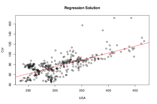
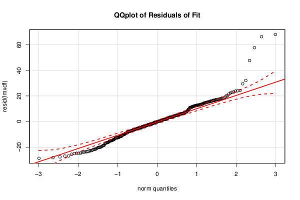
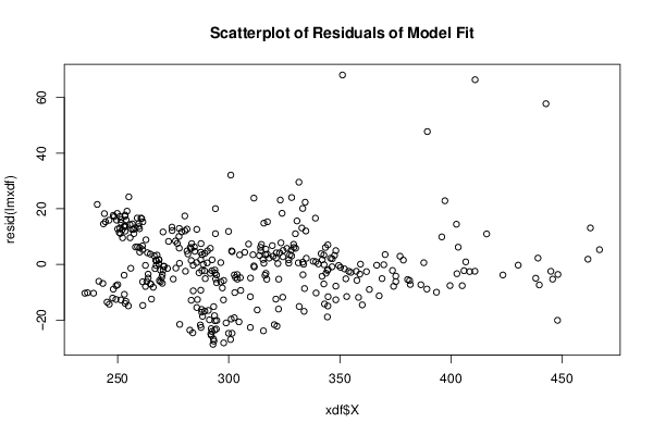
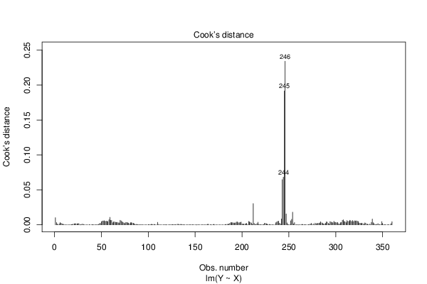
| Title produced by software | Simple Linear Regression | ||||||||||||||||||||||||||||||||||||||||||||||||||||||||||||||||||||||||||||||||||||||||||||||||||||||||||||||||||||||||||||||||||||||||||||||||||||||||||||||||||||||||
| Date of computation | Mon, 10 Dec 2012 13:48:23 -0500 | ||||||||||||||||||||||||||||||||||||||||||||||||||||||||||||||||||||||||||||||||||||||||||||||||||||||||||||||||||||||||||||||||||||||||||||||||||||||||||||||||||||||||
| Cite this page as follows | Statistical Computations at FreeStatistics.org, Office for Research Development and Education, URL https://freestatistics.org/blog/index.php?v=date/2012/Dec/10/t1355165320owr3buy4470g094.htm/, Retrieved Fri, 19 Apr 2024 17:46:17 +0000 | ||||||||||||||||||||||||||||||||||||||||||||||||||||||||||||||||||||||||||||||||||||||||||||||||||||||||||||||||||||||||||||||||||||||||||||||||||||||||||||||||||||||||
| Statistical Computations at FreeStatistics.org, Office for Research Development and Education, URL https://freestatistics.org/blog/index.php?pk=198282, Retrieved Fri, 19 Apr 2024 17:46:17 +0000 | |||||||||||||||||||||||||||||||||||||||||||||||||||||||||||||||||||||||||||||||||||||||||||||||||||||||||||||||||||||||||||||||||||||||||||||||||||||||||||||||||||||||||
| QR Codes: | |||||||||||||||||||||||||||||||||||||||||||||||||||||||||||||||||||||||||||||||||||||||||||||||||||||||||||||||||||||||||||||||||||||||||||||||||||||||||||||||||||||||||
|
| |||||||||||||||||||||||||||||||||||||||||||||||||||||||||||||||||||||||||||||||||||||||||||||||||||||||||||||||||||||||||||||||||||||||||||||||||||||||||||||||||||||||||
| Original text written by user: | |||||||||||||||||||||||||||||||||||||||||||||||||||||||||||||||||||||||||||||||||||||||||||||||||||||||||||||||||||||||||||||||||||||||||||||||||||||||||||||||||||||||||
| IsPrivate? | No (this computation is public) | ||||||||||||||||||||||||||||||||||||||||||||||||||||||||||||||||||||||||||||||||||||||||||||||||||||||||||||||||||||||||||||||||||||||||||||||||||||||||||||||||||||||||
| User-defined keywords | |||||||||||||||||||||||||||||||||||||||||||||||||||||||||||||||||||||||||||||||||||||||||||||||||||||||||||||||||||||||||||||||||||||||||||||||||||||||||||||||||||||||||
| Estimated Impact | 36 | ||||||||||||||||||||||||||||||||||||||||||||||||||||||||||||||||||||||||||||||||||||||||||||||||||||||||||||||||||||||||||||||||||||||||||||||||||||||||||||||||||||||||
Tree of Dependent Computations | |||||||||||||||||||||||||||||||||||||||||||||||||||||||||||||||||||||||||||||||||||||||||||||||||||||||||||||||||||||||||||||||||||||||||||||||||||||||||||||||||||||||||
| Family? (F = Feedback message, R = changed R code, M = changed R Module, P = changed Parameters, D = changed Data) | |||||||||||||||||||||||||||||||||||||||||||||||||||||||||||||||||||||||||||||||||||||||||||||||||||||||||||||||||||||||||||||||||||||||||||||||||||||||||||||||||||||||||
| - [Simple Linear Regression] [] [2012-12-10 18:48:23] [108821faace101f0b67e40eaa0fe63e0] [Current] | |||||||||||||||||||||||||||||||||||||||||||||||||||||||||||||||||||||||||||||||||||||||||||||||||||||||||||||||||||||||||||||||||||||||||||||||||||||||||||||||||||||||||
| Feedback Forum | |||||||||||||||||||||||||||||||||||||||||||||||||||||||||||||||||||||||||||||||||||||||||||||||||||||||||||||||||||||||||||||||||||||||||||||||||||||||||||||||||||||||||
Post a new message | |||||||||||||||||||||||||||||||||||||||||||||||||||||||||||||||||||||||||||||||||||||||||||||||||||||||||||||||||||||||||||||||||||||||||||||||||||||||||||||||||||||||||
Dataset | |||||||||||||||||||||||||||||||||||||||||||||||||||||||||||||||||||||||||||||||||||||||||||||||||||||||||||||||||||||||||||||||||||||||||||||||||||||||||||||||||||||||||
| Dataseries X: | |||||||||||||||||||||||||||||||||||||||||||||||||||||||||||||||||||||||||||||||||||||||||||||||||||||||||||||||||||||||||||||||||||||||||||||||||||||||||||||||||||||||||
1977 1 87.28 255 1977 2 87.28 280.2 1977 3 87.09 299.9 1977 4 86.92 339.2 1977 5 87.59 374.2 1977 6 90.72 393.5 1977 7 90.69 389.2 1977 8 90.3 381.7 1977 9 89.55 375.2 1977 10 88.94 369 1977 11 88.41 357.4 1977 12 87.82 352.1 1978 1 87.07 346.5 1978 2 86.82 342.9 1978 3 86.4 340.3 1978 4 86.02 328.3 1978 5 85.66 322.9 1978 6 85.32 314.3 1978 7 85 308.9 1978 8 84.67 294 1978 9 83.94 285.6 1978 10 82.83 281.2 1978 11 81.95 280.3 1978 12 81.19 278.8 1979 1 80.48 274.5 1979 2 78.86 270.4 1979 3 69.47 263.4 1979 4 68.77 259.9 1979 5 70.06 258 1979 6 73.95 262.7 1979 7 75.8 284.7 1979 8 77.79 311.3 1979 9 81.57 322.1 1979 10 83.07 327 1979 11 84.34 331.3 1979 12 85.1 333.3 1980 1 85.25 321.4 1980 2 84.26 327 1980 3 83.63 320 1980 4 86.44 314.7 1980 5 85.3 316.7 1980 6 84.1 314.4 1980 7 83.36 321.3 1980 8 82.48 318.2 1980 9 81.58 307.2 1980 10 80.47 301.3 1980 11 79.34 287.5 1980 12 82.13 277.7 1981 1 81.69 274.4 1981 2 80.7 258.8 1981 3 79.88 253.3 1981 4 79.16 251 1981 5 78.38 248.4 1981 6 77.42 249.5 1981 7 76.47 246.1 1981 8 75.46 244.5 1981 9 74.48 243.6 1981 10 78.27 244 1981 11 80.7 240.8 1981 12 79.91 249.8 1982 1 78.75 248 1982 2 77.78 259.4 1982 3 81.14 260.5 1982 4 81.08 260.8 1982 5 80.03 261.3 1982 6 78.91 259.5 1982 7 78.01 256.6 1982 8 76.9 257.9 1982 9 75.97 256.5 1982 10 81.93 254.2 1982 11 80.27 253.3 1982 12 78.67 253.8 1983 1 77.42 255.5 1983 2 76.16 257.1 1983 3 74.7 257.3 1983 4 76.39 253.2 1983 5 76.04 252.8 1983 6 74.65 252 1983 7 73.29 250.7 1983 8 71.79 252.2 1983 9 74.39 250 1983 10 74.91 251 1983 11 74.54 253.4 1983 12 73.08 251.2 1984 1 72.75 255.6 1984 2 71.32 261.1 1984 3 70.38 258.9 1984 4 70.35 259.9 1984 5 70.01 261.2 1984 6 69.36 264.7 1984 7 67.77 267.1 1984 8 69.26 266.4 1984 9 69.8 267.7 1984 10 68.38 268.6 1984 11 67.62 267.5 1984 12 68.39 268.5 1985 1 66.95 268.5 1985 2 65.21 270.5 1985 3 66.64 270.9 1985 4 63.45 270.1 1985 5 60.66 269.3 1985 6 62.34 269.8 1985 7 60.32 270.1 1985 8 58.64 264.9 1985 9 60.46 263.7 1985 10 58.59 264.8 1985 11 61.87 263.7 1985 12 61.85 255.9 1986 1 67.44 276.2 1986 2 77.06 360.1 1986 3 91.74 380.5 1986 4 93.15 373.7 1986 5 94.15 369.8 1986 6 93.11 366.6 1986 7 91.51 359.3 1986 8 89.96 345.8 1986 9 88.16 326.2 1986 10 86.98 324.5 1986 11 88.03 328.1 1986 12 86.24 327.5 1987 1 84.65 324.4 1987 2 83.23 316.5 1987 3 81.7 310.9 1987 4 80.25 301.5 1987 5 78.8 291.7 1987 6 77.51 290.4 1987 7 76.2 287.4 1987 8 75.04 277.7 1987 9 74 281.6 1987 10 75.49 288 1987 11 77.14 276 1987 12 76.15 272.9 1988 1 76.27 283 1988 2 78.19 283.3 1988 3 76.49 276.8 1988 4 77.31 284.5 1988 5 76.65 282.7 1988 6 74.99 281.2 1988 7 73.51 287.4 1988 8 72.07 283.1 1988 9 70.59 284 1988 10 71.96 285.5 1988 11 76.29 289.2 1988 12 74.86 292.5 1989 1 74.93 296.4 1989 2 71.9 305.2 1989 3 71.01 303.9 1989 4 77.47 311.5 1989 5 75.78 316.3 1989 6 76.6 316.7 1989 7 76.07 322.5 1989 8 74.57 317.1 1989 9 73.02 309.8 1989 10 72.65 303.8 1989 11 73.16 290.3 1989 12 71.53 293.7 1990 1 69.78 291.7 1990 2 67.98 296.5 1990 3 69.96 289.1 1990 4 72.16 288.5 1990 5 70.47 293.8 1990 6 68.86 297.7 1990 7 67.37 305.4 1990 8 65.87 302.7 1990 9 72.16 302.5 1990 10 71.34 303 1990 11 69.93 294.5 1990 12 68.44 294.1 1991 1 67.16 294.5 1991 2 66.01 297.1 1991 3 67.25 289.4 1991 4 70.91 292.4 1991 5 69.75 287.9 1991 6 68.59 286.6 1991 7 67.48 280.5 1991 8 66.31 272.4 1991 9 64.81 269.2 1991 10 66.58 270.6 1991 11 65.97 267.3 1991 12 64.7 262.5 1992 1 64.7 266.8 1992 2 60.94 268.8 1992 3 59.08 263.1 1992 4 58.42 261.2 1992 5 57.77 266 1992 6 57.11 262.5 1992 7 53.31 265.2 1992 8 49.96 261.3 1992 9 49.4 253.7 1992 10 48.84 249.2 1992 11 48.3 239.1 1992 12 47.74 236.4 1993 1 47.24 235.2 1993 2 46.76 245.2 1993 3 46.29 246.2 1993 4 48.9 247.7 1993 5 49.23 251.4 1993 6 48.53 253.3 1993 7 48.03 254.8 1993 8 54.34 250 1993 9 53.79 249.3 1993 10 53.24 241.5 1993 11 52.96 243.3 1993 12 52.17 248 1994 1 51.7 253 1994 2 58.55 252.9 1994 3 78.2 251.5 1994 4 77.03 251.6 1994 5 76.19 253.5 1994 6 77.15 259.8 1994 7 75.87 334.1 1994 8 95.47 448 1994 9 109.67 445.8 1994 10 112.28 445 1994 11 112.01 448.2 1994 12 107.93 438.2 1995 1 105.96 439.8 1995 2 105.06 423.4 1995 3 102.98 410.8 1995 4 102.2 408.4 1995 5 105.23 406.7 1995 6 101.85 405.9 1995 7 99.89 402.7 1995 8 96.23 405.1 1995 9 94.76 399.6 1995 10 91.51 386.5 1995 11 91.63 381.4 1995 12 91.54 375.2 1996 1 85.23 357.7 1996 2 87.83 359 1996 3 87.38 355 1996 4 84.44 352.7 1996 5 85.19 344.4 1996 6 84.03 343.8 1996 7 86.73 338 1996 8 102.52 339 1996 9 104.45 333.3 1996 10 106.98 334.4 1996 11 107.02 328.3 1996 12 99.26 330.7 1997 1 94.45 330 1997 2 113.44 331.6 1997 3 157.33 351.2 1997 4 147.38 389.4 1997 5 171.89 410.9 1997 6 171.95 442.8 1997 7 132.71 462.8 1997 8 126.02 466.9 1997 9 121.18 461.7 1997 10 115.45 439.2 1997 11 110.48 430.3 1997 12 117.85 416.1 1998 1 117.63 402.5 1998 2 124.65 397.3 1998 3 109.59 403.3 1998 4 111.27 395.9 1998 5 99.78 387.8 1998 6 98.21 378.6 1998 7 99.2 377.1 1998 8 97.97 370.4 1998 9 89.55 362 1998 10 87.91 350.3 1998 11 93.34 348.2 1998 12 94.42 344.6 1999 1 93.2 343.5 1999 2 90.29 342.8 1999 3 91.46 347.6 1999 4 89.98 346.6 1999 5 88.35 349.5 1999 6 88.41 342.1 1999 7 82.44 342 1999 8 79.89 342.8 1999 9 75.69 339.3 1999 10 75.66 348.2 1999 11 84.5 333.7 1999 12 96.73 334.7 2000 1 87.48 354 2000 2 82.39 367.7 2000 3 83.48 363.3 2000 4 79.31 358.4 2000 5 78.16 353.1 2000 6 72.77 343.1 2000 7 72.45 344.6 2000 8 68.46 344.4 2000 9 67.62 333.9 2000 10 68.76 331.7 2000 11 70.07 324.3 2000 12 68.55 321.2 2001 1 65.3 322.4 2001 2 58.96 321.7 2001 3 59.17 320.5 2001 4 62.37 312.8 2001 5 66.28 309.7 2001 6 55.62 315.6 2001 7 55.23 309.7 2001 8 55.85 304.6 2001 9 56.75 302.5 2001 10 50.89 301.5 2001 11 53.88 298.8 2001 12 52.95 291.3 2002 1 55.08 293.6 2002 2 53.61 294.6 2002 3 58.78 285.9 2002 4 61.85 297.6 2002 5 55.91 301.1 2002 6 53.32 293.8 2002 7 46.41 297.7 2002 8 44.57 292.9 2002 9 50 292.1 2002 10 50 287.2 2002 11 53.36 288.2 2002 12 46.23 283.8 2003 1 50.45 299.9 2003 2 49.07 292.4 2003 3 45.85 293.3 2003 4 48.45 300.8 2003 5 49.96 293.7 2003 6 46.53 293.1 2003 7 50.51 294.4 2003 8 47.58 292.1 2003 9 48.05 291.9 2003 10 46.84 282.5 2003 11 47.67 277.9 2003 12 49.16 287.5 2004 1 55.54 289.2 2004 2 55.82 285.6 2004 3 58.22 293.2 2004 4 56.19 290.8 2004 5 57.77 283.1 2004 6 63.19 275 2004 7 54.76 287.8 2004 8 55.74 287.8 2004 9 62.54 287.4 2004 10 61.39 284 2004 11 69.6 277.8 2004 12 79.23 277.6 2005 1 80 304.9 2005 2 93.68 294 2005 3 107.63 300.9 2005 4 100.18 324 2005 5 97.3 332.9 2005 6 90.45 341.6 2005 7 80.64 333.4 2005 8 80.58 348.2 2005 9 75.82 344.7 2005 10 85.59 344.7 2005 11 89.35 329.3 2005 12 89.42 323.5 2006 1 104.73 323.2 2006 2 95.32 317.4 2006 3 89.27 330.1 2006 4 90.44 329.2 2006 5 86.97 334.9 2006 6 79.98 315.8 2006 7 81.22 315.4 2006 8 87.35 319.6 2006 9 83.64 317.3 2006 10 82.22 313.8 2006 11 94.4 315.8 2006 12 102.18 311.3 | |||||||||||||||||||||||||||||||||||||||||||||||||||||||||||||||||||||||||||||||||||||||||||||||||||||||||||||||||||||||||||||||||||||||||||||||||||||||||||||||||||||||||
Tables (Output of Computation) | |||||||||||||||||||||||||||||||||||||||||||||||||||||||||||||||||||||||||||||||||||||||||||||||||||||||||||||||||||||||||||||||||||||||||||||||||||||||||||||||||||||||||
| |||||||||||||||||||||||||||||||||||||||||||||||||||||||||||||||||||||||||||||||||||||||||||||||||||||||||||||||||||||||||||||||||||||||||||||||||||||||||||||||||||||||||
Figures (Output of Computation) | |||||||||||||||||||||||||||||||||||||||||||||||||||||||||||||||||||||||||||||||||||||||||||||||||||||||||||||||||||||||||||||||||||||||||||||||||||||||||||||||||||||||||
Input Parameters & R Code | |||||||||||||||||||||||||||||||||||||||||||||||||||||||||||||||||||||||||||||||||||||||||||||||||||||||||||||||||||||||||||||||||||||||||||||||||||||||||||||||||||||||||
| Parameters (Session): | |||||||||||||||||||||||||||||||||||||||||||||||||||||||||||||||||||||||||||||||||||||||||||||||||||||||||||||||||||||||||||||||||||||||||||||||||||||||||||||||||||||||||
| par1 = 3 ; par2 = 4 ; par3 = TRUE ; | |||||||||||||||||||||||||||||||||||||||||||||||||||||||||||||||||||||||||||||||||||||||||||||||||||||||||||||||||||||||||||||||||||||||||||||||||||||||||||||||||||||||||
| Parameters (R input): | |||||||||||||||||||||||||||||||||||||||||||||||||||||||||||||||||||||||||||||||||||||||||||||||||||||||||||||||||||||||||||||||||||||||||||||||||||||||||||||||||||||||||
| par1 = 3 ; par2 = 4 ; par3 = TRUE ; | |||||||||||||||||||||||||||||||||||||||||||||||||||||||||||||||||||||||||||||||||||||||||||||||||||||||||||||||||||||||||||||||||||||||||||||||||||||||||||||||||||||||||
| R code (references can be found in the software module): | |||||||||||||||||||||||||||||||||||||||||||||||||||||||||||||||||||||||||||||||||||||||||||||||||||||||||||||||||||||||||||||||||||||||||||||||||||||||||||||||||||||||||
cat1 <- as.numeric(par1) | |||||||||||||||||||||||||||||||||||||||||||||||||||||||||||||||||||||||||||||||||||||||||||||||||||||||||||||||||||||||||||||||||||||||||||||||||||||||||||||||||||||||||