Free Statistics
of Irreproducible Research!
Description of Statistical Computation | |||||||||||||||||||||||||||||||||||||||||||||||||||||||||||||||||||||||||||||||||
|---|---|---|---|---|---|---|---|---|---|---|---|---|---|---|---|---|---|---|---|---|---|---|---|---|---|---|---|---|---|---|---|---|---|---|---|---|---|---|---|---|---|---|---|---|---|---|---|---|---|---|---|---|---|---|---|---|---|---|---|---|---|---|---|---|---|---|---|---|---|---|---|---|---|---|---|---|---|---|---|---|---|
| Author's title | |||||||||||||||||||||||||||||||||||||||||||||||||||||||||||||||||||||||||||||||||
| Author | *The author of this computation has been verified* | ||||||||||||||||||||||||||||||||||||||||||||||||||||||||||||||||||||||||||||||||
| R Software Module | rwasp_bootstrapplot.wasp | ||||||||||||||||||||||||||||||||||||||||||||||||||||||||||||||||||||||||||||||||
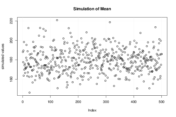
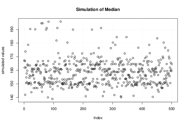
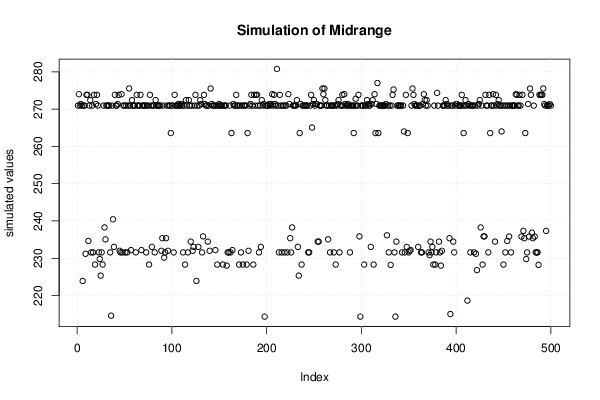
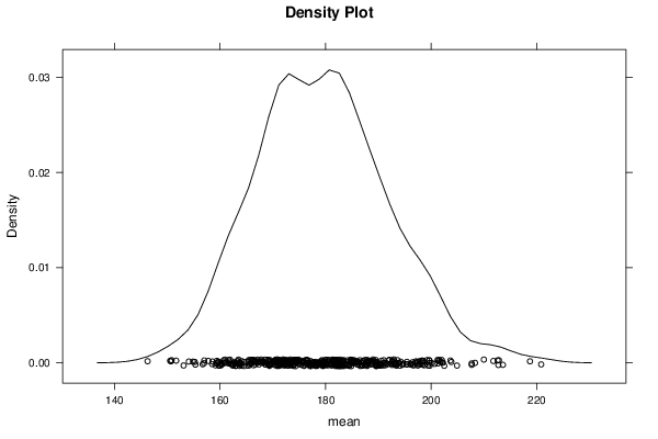
| Title produced by software | Blocked Bootstrap Plot - Central Tendency | ||||||||||||||||||||||||||||||||||||||||||||||||||||||||||||||||||||||||||||||||
| Date of computation | Sun, 09 Dec 2012 10:29:42 -0500 | ||||||||||||||||||||||||||||||||||||||||||||||||||||||||||||||||||||||||||||||||
| Cite this page as follows | Statistical Computations at FreeStatistics.org, Office for Research Development and Education, URL https://freestatistics.org/blog/index.php?v=date/2012/Dec/09/t1355067350rkgof1vv8xjxrga.htm/, Retrieved Fri, 26 Apr 2024 20:51:01 +0000 | ||||||||||||||||||||||||||||||||||||||||||||||||||||||||||||||||||||||||||||||||
| Statistical Computations at FreeStatistics.org, Office for Research Development and Education, URL https://freestatistics.org/blog/index.php?pk=197931, Retrieved Fri, 26 Apr 2024 20:51:01 +0000 | |||||||||||||||||||||||||||||||||||||||||||||||||||||||||||||||||||||||||||||||||
| QR Codes: | |||||||||||||||||||||||||||||||||||||||||||||||||||||||||||||||||||||||||||||||||
|
| |||||||||||||||||||||||||||||||||||||||||||||||||||||||||||||||||||||||||||||||||
| Original text written by user: | |||||||||||||||||||||||||||||||||||||||||||||||||||||||||||||||||||||||||||||||||
| IsPrivate? | No (this computation is public) | ||||||||||||||||||||||||||||||||||||||||||||||||||||||||||||||||||||||||||||||||
| User-defined keywords | |||||||||||||||||||||||||||||||||||||||||||||||||||||||||||||||||||||||||||||||||
| Estimated Impact | 115 | ||||||||||||||||||||||||||||||||||||||||||||||||||||||||||||||||||||||||||||||||
Tree of Dependent Computations | |||||||||||||||||||||||||||||||||||||||||||||||||||||||||||||||||||||||||||||||||
| Family? (F = Feedback message, R = changed R code, M = changed R Module, P = changed Parameters, D = changed Data) | |||||||||||||||||||||||||||||||||||||||||||||||||||||||||||||||||||||||||||||||||
| - [Bivariate Data Series] [Bivariate dataset] [2008-01-05 23:51:08] [74be16979710d4c4e7c6647856088456] - RMPD [Blocked Bootstrap Plot - Central Tendency] [Colombia Coffee] [2008-01-07 10:26:26] [74be16979710d4c4e7c6647856088456] - RM D [Blocked Bootstrap Plot - Central Tendency] [Paper] [2012-12-09 15:29:42] [38c0fff34b8aa23b45468de8b641bfee] [Current] - D [Blocked Bootstrap Plot - Central Tendency] [paper] [2012-12-16 11:28:04] [fa543719fe3f8358943b948de15add90] - RMPD [Histogram] [paper] [2012-12-16 11:35:45] [fa543719fe3f8358943b948de15add90] | |||||||||||||||||||||||||||||||||||||||||||||||||||||||||||||||||||||||||||||||||
| Feedback Forum | |||||||||||||||||||||||||||||||||||||||||||||||||||||||||||||||||||||||||||||||||
Post a new message | |||||||||||||||||||||||||||||||||||||||||||||||||||||||||||||||||||||||||||||||||
Dataset | |||||||||||||||||||||||||||||||||||||||||||||||||||||||||||||||||||||||||||||||||
| Dataseries X: | |||||||||||||||||||||||||||||||||||||||||||||||||||||||||||||||||||||||||||||||||
115.01 124.56 128.60 131.54 124.93 126.77 128.97 149.91 149.55 149.91 159.47 162.04 163.88 166.82 173.80 172.06 178.21 174.53 176.37 168.65 166.82 164.24 163.51 164.61 163.51 164.61 167.92 160.94 156.53 159.47 149.18 135.58 124.93 116.84 114.27 114.64 112.80 113.17 111.33 113.91 119.42 120.89 122.04 120.15 118.21 125.33 135.37 146.89 149.54 160.84 169.95 177.13 169.35 159.93 149.69 148.67 136.32 128.17 138.74 140.58 147.57 147.83 155.65 148.88 147.90 141.99 136.58 121.82 127.52 129.80 131.29 135.96 146.50 158.65 153.21 147.04 141.04 140.45 140.15 139.30 137.60 146.02 158.79 167.19 161.99 164.62 156.21 154.42 150.39 148.98 158.61 169.98 190.09 184.39 193.67 203.79 204.07 208.92 206.88 218.89 215.52 251.66 262.11 227.27 202.60 191.63 178.71 178.32 176.41 175.70 175.73 172.35 176.61 183.49 172.59 148.39 138.31 150.61 151.74 151.66 149.88 144.62 137.10 140.05 138.92 130.15 128.92 120.64 118.54 107.95 107.93 126.54 130.21 126.21 125.29 117.03 117.34 113.87 113.00 111.41 103.02 111.41 113.19 108.10 108.80 102.16 105.83 108.41 105.70 105.11 110.78 113.51 108.98 108.28 117.49 128.22 127.73 128.01 132.84 128.12 130.28 129.30 135.00 127.23 123.79 121.92 122.03 123.34 125.27 122.53 125.31 123.28 122.56 123.72 121.46 132.03 149.30 161.26 187.84 190.32 176.26 168.98 149.60 150.84 141.81 138.62 141.96 131.35 131.62 148.72 145.62 147.46 160.55 165.57 166.33 161.39 166.28 166.58 163.73 154.74 150.60 141.29 151.03 150.15 156.57 153.87 153.59 151.30 150.99 140.88 144.25 141.93 143.87 149.36 159.71 167.83 161.12 164.44 167.16 179.84 174.44 180.35 193.17 195.16 202.43 189.91 195.98 212.09 205.81 204.31 196.07 199.98 199.10 198.31 195.72 223.04 238.41 259.73 326.54 335.15 321.81 368.62 369.59 425.00 439.72 362.23 328.76 348.55 328.18 329.34 295.55 237.38 226.85 220.14 239.36 224.69 230.98 233.47 256.70 253.41 224.95 210.37 191.09 198.85 211.04 206.25 201.51 194.54 191.07 192.82 181.88 157.67 195.82 246.25 271.69 270.23 274.08 306.53 326.55 348.15 316.75 336.12 354.47 326.43 303.88 327.07 315.92 289.01 281.01 269.03 274.89 277.77 283.88 266.32 264.36 276.19 345.69 349.40 353.42 358.20 361.00 | |||||||||||||||||||||||||||||||||||||||||||||||||||||||||||||||||||||||||||||||||
Tables (Output of Computation) | |||||||||||||||||||||||||||||||||||||||||||||||||||||||||||||||||||||||||||||||||
| |||||||||||||||||||||||||||||||||||||||||||||||||||||||||||||||||||||||||||||||||
Figures (Output of Computation) | |||||||||||||||||||||||||||||||||||||||||||||||||||||||||||||||||||||||||||||||||
Input Parameters & R Code | |||||||||||||||||||||||||||||||||||||||||||||||||||||||||||||||||||||||||||||||||
| Parameters (Session): | |||||||||||||||||||||||||||||||||||||||||||||||||||||||||||||||||||||||||||||||||
| par1 = 500 ; par2 = 12 ; | |||||||||||||||||||||||||||||||||||||||||||||||||||||||||||||||||||||||||||||||||
| Parameters (R input): | |||||||||||||||||||||||||||||||||||||||||||||||||||||||||||||||||||||||||||||||||
| par1 = 500 ; par2 = 12 ; | |||||||||||||||||||||||||||||||||||||||||||||||||||||||||||||||||||||||||||||||||
| R code (references can be found in the software module): | |||||||||||||||||||||||||||||||||||||||||||||||||||||||||||||||||||||||||||||||||
par1 <- as.numeric(par1) | |||||||||||||||||||||||||||||||||||||||||||||||||||||||||||||||||||||||||||||||||