Free Statistics
of Irreproducible Research!
Description of Statistical Computation | |||||||||||||||||||||||||||||||||||||||
|---|---|---|---|---|---|---|---|---|---|---|---|---|---|---|---|---|---|---|---|---|---|---|---|---|---|---|---|---|---|---|---|---|---|---|---|---|---|---|---|
| Author's title | |||||||||||||||||||||||||||||||||||||||
| Author | *Unverified author* | ||||||||||||||||||||||||||||||||||||||
| R Software Module | rwasp_fitdistrweibull.wasp | ||||||||||||||||||||||||||||||||||||||
| Title produced by software | Maximum-likelihood Fitting - Weibull Distribution | ||||||||||||||||||||||||||||||||||||||
| Date of computation | Thu, 06 Dec 2012 19:31:39 -0500 | ||||||||||||||||||||||||||||||||||||||
| Cite this page as follows | Statistical Computations at FreeStatistics.org, Office for Research Development and Education, URL https://freestatistics.org/blog/index.php?v=date/2012/Dec/06/t1354840573qt2bn06axo4py09.htm/, Retrieved Sat, 27 Apr 2024 00:20:45 +0000 | ||||||||||||||||||||||||||||||||||||||
| Statistical Computations at FreeStatistics.org, Office for Research Development and Education, URL https://freestatistics.org/blog/index.php?pk=197255, Retrieved Sat, 27 Apr 2024 00:20:45 +0000 | |||||||||||||||||||||||||||||||||||||||
| QR Codes: | |||||||||||||||||||||||||||||||||||||||
|
| |||||||||||||||||||||||||||||||||||||||
| Original text written by user: | target conc. 0.15% | ||||||||||||||||||||||||||||||||||||||
| IsPrivate? | No (this computation is public) | ||||||||||||||||||||||||||||||||||||||
| User-defined keywords | Forensic alcohol analysis (FAA) Proficiency testing Crime Labs in California USA blood pool November 2012, CDPH ASAS | ||||||||||||||||||||||||||||||||||||||
| Estimated Impact | 123 | ||||||||||||||||||||||||||||||||||||||
Tree of Dependent Computations | |||||||||||||||||||||||||||||||||||||||
| Family? (F = Feedback message, R = changed R code, M = changed R Module, P = changed Parameters, D = changed Data) | |||||||||||||||||||||||||||||||||||||||
| - [Maximum-likelihood Fitting - Weibull Distribution] [CDPH pool 10082-W...] [2012-12-07 00:31:39] [d41d8cd98f00b204e9800998ecf8427e] [Current] - PD [Maximum-likelihood Fitting - Weibull Distribution] [CDPH pool 10082-W...] [2012-12-11 18:47:19] [74be16979710d4c4e7c6647856088456] - RMPD [Bootstrap Plot - Central Tendency] [CDPH pool 10152 b...] [2012-12-11 19:00:00] [74be16979710d4c4e7c6647856088456] - RMPD [Kernel Density Estimation] [CDPH pool 10152 G...] [2012-12-11 19:59:00] [74be16979710d4c4e7c6647856088456] - RMPD [Bootstrap Plot - Central Tendency] [CDPH pool 10152 b...] [2012-12-11 21:29:01] [74be16979710d4c4e7c6647856088456] - R PD [Bootstrap Plot - Central Tendency] [CDPH pool 06173 b...] [2013-08-16 00:46:13] [74be16979710d4c4e7c6647856088456] - R D [Maximum-likelihood Fitting - Weibull Distribution] [CDPH pool 10152-W...] [2012-12-11 22:10:22] [74be16979710d4c4e7c6647856088456] | |||||||||||||||||||||||||||||||||||||||
| Feedback Forum | |||||||||||||||||||||||||||||||||||||||
Post a new message | |||||||||||||||||||||||||||||||||||||||
Dataset | |||||||||||||||||||||||||||||||||||||||
| Dataseries X: | |||||||||||||||||||||||||||||||||||||||
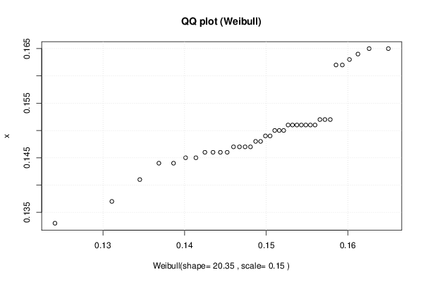
0.133 0.137 0.141 0.144 0.144 0.145 0.145 0.146 0.146 0.146 0.146 0.147 0.147 0.147 0.147 0.148 0.148 0.149 0.149 0.150 0.150 0.150 0.151 0.151 0.151 0.151 0.151 0.151 0.151 0.152 0.152 0.152 0.162 0.162 0.163 0.164 0.165 0.165 | |||||||||||||||||||||||||||||||||||||||
Tables (Output of Computation) | |||||||||||||||||||||||||||||||||||||||
| |||||||||||||||||||||||||||||||||||||||
Figures (Output of Computation) | |||||||||||||||||||||||||||||||||||||||
Input Parameters & R Code | |||||||||||||||||||||||||||||||||||||||
| Parameters (Session): | |||||||||||||||||||||||||||||||||||||||
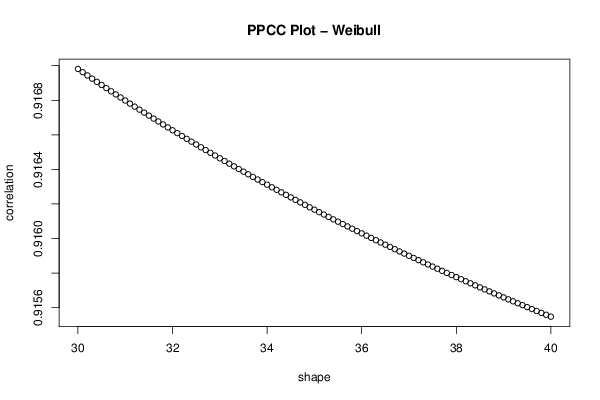
| par1 = 30 ; par2 = 40 ; | |||||||||||||||||||||||||||||||||||||||
| Parameters (R input): | |||||||||||||||||||||||||||||||||||||||
| par1 = 30 ; par2 = 40 ; | |||||||||||||||||||||||||||||||||||||||
| R code (references can be found in the software module): | |||||||||||||||||||||||||||||||||||||||
library(MASS) | |||||||||||||||||||||||||||||||||||||||