Free Statistics
of Irreproducible Research!
Description of Statistical Computation | |||||||||||||||||||||||||||||||||||||||||||||||||||||||||||||||||||||||||||||||||
|---|---|---|---|---|---|---|---|---|---|---|---|---|---|---|---|---|---|---|---|---|---|---|---|---|---|---|---|---|---|---|---|---|---|---|---|---|---|---|---|---|---|---|---|---|---|---|---|---|---|---|---|---|---|---|---|---|---|---|---|---|---|---|---|---|---|---|---|---|---|---|---|---|---|---|---|---|---|---|---|---|---|
| Author's title | |||||||||||||||||||||||||||||||||||||||||||||||||||||||||||||||||||||||||||||||||
| Author | *Unverified author* | ||||||||||||||||||||||||||||||||||||||||||||||||||||||||||||||||||||||||||||||||
| R Software Module | rwasp_bootstrapplot.wasp | ||||||||||||||||||||||||||||||||||||||||||||||||||||||||||||||||||||||||||||||||
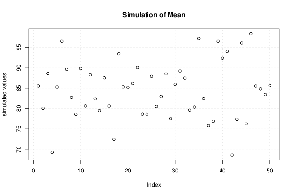
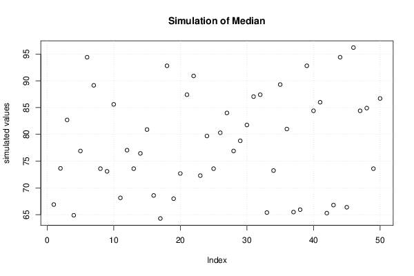
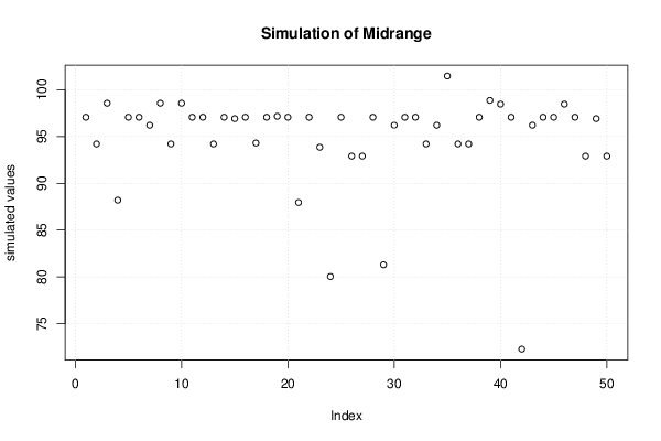
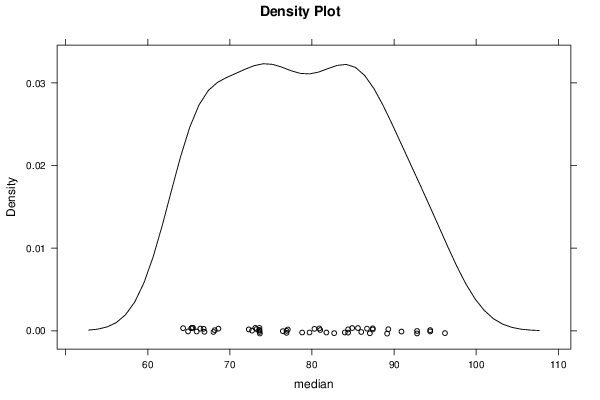
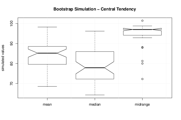
| Title produced by software | Blocked Bootstrap Plot - Central Tendency | ||||||||||||||||||||||||||||||||||||||||||||||||||||||||||||||||||||||||||||||||
| Date of computation | Tue, 04 Dec 2012 17:05:27 -0500 | ||||||||||||||||||||||||||||||||||||||||||||||||||||||||||||||||||||||||||||||||
| Cite this page as follows | Statistical Computations at FreeStatistics.org, Office for Research Development and Education, URL https://freestatistics.org/blog/index.php?v=date/2012/Dec/04/t135465876405ekev2vg7a408d.htm/, Retrieved Thu, 25 Apr 2024 12:49:48 +0000 | ||||||||||||||||||||||||||||||||||||||||||||||||||||||||||||||||||||||||||||||||
| Statistical Computations at FreeStatistics.org, Office for Research Development and Education, URL https://freestatistics.org/blog/index.php?pk=196672, Retrieved Thu, 25 Apr 2024 12:49:48 +0000 | |||||||||||||||||||||||||||||||||||||||||||||||||||||||||||||||||||||||||||||||||
| QR Codes: | |||||||||||||||||||||||||||||||||||||||||||||||||||||||||||||||||||||||||||||||||
|
| |||||||||||||||||||||||||||||||||||||||||||||||||||||||||||||||||||||||||||||||||
| Original text written by user: | |||||||||||||||||||||||||||||||||||||||||||||||||||||||||||||||||||||||||||||||||
| IsPrivate? | No (this computation is public) | ||||||||||||||||||||||||||||||||||||||||||||||||||||||||||||||||||||||||||||||||
| User-defined keywords | |||||||||||||||||||||||||||||||||||||||||||||||||||||||||||||||||||||||||||||||||
| Estimated Impact | 81 | ||||||||||||||||||||||||||||||||||||||||||||||||||||||||||||||||||||||||||||||||
Tree of Dependent Computations | |||||||||||||||||||||||||||||||||||||||||||||||||||||||||||||||||||||||||||||||||
| Family? (F = Feedback message, R = changed R code, M = changed R Module, P = changed Parameters, D = changed Data) | |||||||||||||||||||||||||||||||||||||||||||||||||||||||||||||||||||||||||||||||||
| - [Blocked Bootstrap Plot - Central Tendency] [] [2012-12-04 22:05:27] [e3cb5e3bac8dbaf27c4382afdd169712] [Current] - RMPD [Bootstrap Plot - Central Tendency] [] [2012-12-14 20:18:15] [873b10c79bed0b14ae85834791a7b7d7] - R PD [Bootstrap Plot - Central Tendency] [] [2012-12-14 20:25:30] [873b10c79bed0b14ae85834791a7b7d7] - P [Bootstrap Plot - Central Tendency] [] [2012-12-14 20:28:53] [873b10c79bed0b14ae85834791a7b7d7] - RMPD [Variability] [] [2012-12-14 21:36:17] [873b10c79bed0b14ae85834791a7b7d7] - RMPD [Standard Deviation Plot] [] [2012-12-14 21:38:46] [873b10c79bed0b14ae85834791a7b7d7] - RMPD [Standard Deviation-Mean Plot] [] [2012-12-14 21:40:37] [873b10c79bed0b14ae85834791a7b7d7] - D [Variability] [] [2012-12-14 21:42:24] [873b10c79bed0b14ae85834791a7b7d7] - RMPD [Standard Deviation Plot] [] [2012-12-14 21:43:47] [873b10c79bed0b14ae85834791a7b7d7] - RMPD [Standard Deviation-Mean Plot] [] [2012-12-14 21:45:02] [873b10c79bed0b14ae85834791a7b7d7] - RMPD [Classical Decomposition] [] [2012-12-14 21:47:32] [873b10c79bed0b14ae85834791a7b7d7] - RMPD [Classical Decomposition] [] [2012-12-14 21:49:45] [873b10c79bed0b14ae85834791a7b7d7] | |||||||||||||||||||||||||||||||||||||||||||||||||||||||||||||||||||||||||||||||||
| Feedback Forum | |||||||||||||||||||||||||||||||||||||||||||||||||||||||||||||||||||||||||||||||||
Post a new message | |||||||||||||||||||||||||||||||||||||||||||||||||||||||||||||||||||||||||||||||||
Dataset | |||||||||||||||||||||||||||||||||||||||||||||||||||||||||||||||||||||||||||||||||
| Dataseries X: | |||||||||||||||||||||||||||||||||||||||||||||||||||||||||||||||||||||||||||||||||
65 65,3 62,9 63,5 62,1 59,3 61,6 61,5 60,1 59,5 62,7 65,5 63,8 63,8 62,7 62,3 62,4 64,8 66,4 65,1 67,4 68,8 68,6 71,5 75 84,3 84 79,1 78,8 82,7 85,3 84,5 80,8 70,1 68,2 68,1 72,3 73,1 71,5 74,1 80,3 80,6 81,4 87,4 89,3 93,2 92,8 96,8 100,3 95,6 89 87,4 86,7 92,8 98,6 100,8 105,5 107,8 113,7 120,3 126,5 134,8 134,5 133,1 128,8 127,1 129,1 128,4 126,5 117,1 114,2 109,1 | |||||||||||||||||||||||||||||||||||||||||||||||||||||||||||||||||||||||||||||||||
Tables (Output of Computation) | |||||||||||||||||||||||||||||||||||||||||||||||||||||||||||||||||||||||||||||||||
| |||||||||||||||||||||||||||||||||||||||||||||||||||||||||||||||||||||||||||||||||
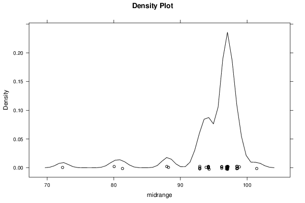
Figures (Output of Computation) | |||||||||||||||||||||||||||||||||||||||||||||||||||||||||||||||||||||||||||||||||
Input Parameters & R Code | |||||||||||||||||||||||||||||||||||||||||||||||||||||||||||||||||||||||||||||||||
| Parameters (Session): | |||||||||||||||||||||||||||||||||||||||||||||||||||||||||||||||||||||||||||||||||
| par1 = 50 ; par2 = 12 ; | |||||||||||||||||||||||||||||||||||||||||||||||||||||||||||||||||||||||||||||||||
| Parameters (R input): | |||||||||||||||||||||||||||||||||||||||||||||||||||||||||||||||||||||||||||||||||
| par1 = 50 ; par2 = 12 ; | |||||||||||||||||||||||||||||||||||||||||||||||||||||||||||||||||||||||||||||||||
| R code (references can be found in the software module): | |||||||||||||||||||||||||||||||||||||||||||||||||||||||||||||||||||||||||||||||||
par1 <- as.numeric(par1) | |||||||||||||||||||||||||||||||||||||||||||||||||||||||||||||||||||||||||||||||||