Free Statistics

of Irreproducible Research!

Author's title

Author*The author of this computation has been verified*
R Software Modulerwasp_arimaforecasting.wasp
Title produced by softwareARIMA Forecasting
Date of computationTue, 04 Dec 2012 13:38:36 -0500
Cite this page as followsStatistical Computations at FreeStatistics.org, Office for Research Development and Education, URL https://freestatistics.org/blog/index.php?v=date/2012/Dec/04/t1354646329hdtolvcicsyj6f8.htm/, Retrieved Thu, 18 Apr 2024 18:12:01 +0000
Statistical Computations at FreeStatistics.org, Office for Research Development and Education, URL https://freestatistics.org/blog/index.php?pk=196487, Retrieved Thu, 18 Apr 2024 18:12:01 +0000
QR Codes:

Original text written by user:
IsPrivate?No (this computation is public)
User-defined keywords
Estimated Impact103
Family? (F = Feedback message, R = changed R code, M = changed R Module, P = changed Parameters, D = changed Data)
-     [Univariate Data Series] [data set] [2008-12-01 19:54:57] [b98453cac15ba1066b407e146608df68]
- RMP   [Standard Deviation-Mean Plot] [Unemployment] [2010-11-29 10:34:47] [b98453cac15ba1066b407e146608df68]
- RMP     [ARIMA Forecasting] [Unemployment] [2010-11-29 20:46:45] [b98453cac15ba1066b407e146608df68]
- R PD        [ARIMA Forecasting] [ARIMA Forecasting] [2012-12-04 18:38:36] [86f0addf4b5362ca5a545029cdfac14b] [Current]
- R P           [ARIMA Forecasting] [ARIMA Forecasting] [2012-12-15 11:36:05] [74be16979710d4c4e7c6647856088456]
- R P           [ARIMA Forecasting] [Paper2012: ARIMA] [2012-12-20 11:20:35] [f055db2f1c47e4197bf514e64f7886e5]
Feedback Forum

Post a new message
Dataseries X:
46
62
66
59
58
61
41
27
58
70
49
59
44
36
72
45
56
54
53
35
61
52
47
51
52
63
74
45
51
64
36
30
55
64
39
40
63
45
59
55
40
64
27
28
45
57
45
69
60
56
58
50
51
53
37
22
55
70
62
58
39
49
58
47
42
62
39
40
72
70
54
65


Summary of computational transaction
Raw Inputview raw input (R code)
Raw Outputview raw output of R engine
Computing time3 seconds
R Server'George Udny Yule' @ yule.wessa.net

\begin{tabular}{lllllllll}
\hline
Summary of computational transaction \tabularnewline
Raw Input & view raw input (R code)  \tabularnewline
Raw Output & view raw output of R engine  \tabularnewline
Computing time & 3 seconds \tabularnewline
R Server & 'George Udny Yule' @ yule.wessa.net \tabularnewline
\hline
\end{tabular}
%Source: https://freestatistics.org/blog/index.php?pk=196487&T=0

[TABLE]
[ROW][C]Summary of computational transaction[/C][/ROW]
[ROW][C]Raw Input[/C][C]view raw input (R code) [/C][/ROW]
[ROW][C]Raw Output[/C][C]view raw output of R engine [/C][/ROW]
[ROW][C]Computing time[/C][C]3 seconds[/C][/ROW]
[ROW][C]R Server[/C][C]'George Udny Yule' @ yule.wessa.net[/C][/ROW]
[/TABLE]
Source: https://freestatistics.org/blog/index.php?pk=196487&T=0

Globally Unique Identifier (entire table): ba.freestatistics.org/blog/index.php?pk=196487&T=0

As an alternative you can also use a QR Code:  

The GUIDs for individual cells are displayed in the table below:

Summary of computational transaction
Raw Inputview raw input (R code)
Raw Outputview raw output of R engine
Computing time3 seconds
R Server'George Udny Yule' @ yule.wessa.net


Univariate ARIMA Extrapolation Forecast
timeY[t]F[t]95% LB95% UBp-value(H0: Y[t] = F[t])P(F[t]>Y[t-1])P(F[t]>Y[t-s])P(F[t]>Y[60])
4869-------
4960-------
5056-------
5158-------
5250-------
5351-------
5453-------
5537-------
5622-------
5755-------
5870-------
5962-------
6058-------
613964.670844.989784.35190.00530.74680.67910.7468
624951.390431.710671.07020.40590.89140.32310.2552
635859.420939.391479.45050.44470.84610.55530.5553
644753.079233.034573.12380.27610.31520.61830.3152
654246.150526.054766.24630.34280.4670.31810.1239
666259.037338.917479.15710.38640.95150.72180.5402
673932.605412.455852.7550.2670.00210.33450.0068
684025.55075.374945.72640.08020.09570.63498e-04
697250.599630.396870.80240.01890.84810.33470.2364
707064.107543.878384.33680.2840.22220.2840.723
715454.119733.863874.37550.49540.06220.22290.3537
726564.035843.753484.31810.46290.83390.72010.7201

\begin{tabular}{lllllllll}
\hline
Univariate ARIMA Extrapolation Forecast \tabularnewline
time & Y[t] & F[t] & 95% LB & 95% UB & p-value(H0: Y[t] = F[t]) & P(F[t]>Y[t-1]) & P(F[t]>Y[t-s]) & P(F[t]>Y[60]) \tabularnewline
48 & 69 & - & - & - & - & - & - & - \tabularnewline
49 & 60 & - & - & - & - & - & - & - \tabularnewline
50 & 56 & - & - & - & - & - & - & - \tabularnewline
51 & 58 & - & - & - & - & - & - & - \tabularnewline
52 & 50 & - & - & - & - & - & - & - \tabularnewline
53 & 51 & - & - & - & - & - & - & - \tabularnewline
54 & 53 & - & - & - & - & - & - & - \tabularnewline
55 & 37 & - & - & - & - & - & - & - \tabularnewline
56 & 22 & - & - & - & - & - & - & - \tabularnewline
57 & 55 & - & - & - & - & - & - & - \tabularnewline
58 & 70 & - & - & - & - & - & - & - \tabularnewline
59 & 62 & - & - & - & - & - & - & - \tabularnewline
60 & 58 & - & - & - & - & - & - & - \tabularnewline
61 & 39 & 64.6708 & 44.9897 & 84.3519 & 0.0053 & 0.7468 & 0.6791 & 0.7468 \tabularnewline
62 & 49 & 51.3904 & 31.7106 & 71.0702 & 0.4059 & 0.8914 & 0.3231 & 0.2552 \tabularnewline
63 & 58 & 59.4209 & 39.3914 & 79.4505 & 0.4447 & 0.8461 & 0.5553 & 0.5553 \tabularnewline
64 & 47 & 53.0792 & 33.0345 & 73.1238 & 0.2761 & 0.3152 & 0.6183 & 0.3152 \tabularnewline
65 & 42 & 46.1505 & 26.0547 & 66.2463 & 0.3428 & 0.467 & 0.3181 & 0.1239 \tabularnewline
66 & 62 & 59.0373 & 38.9174 & 79.1571 & 0.3864 & 0.9515 & 0.7218 & 0.5402 \tabularnewline
67 & 39 & 32.6054 & 12.4558 & 52.755 & 0.267 & 0.0021 & 0.3345 & 0.0068 \tabularnewline
68 & 40 & 25.5507 & 5.3749 & 45.7264 & 0.0802 & 0.0957 & 0.6349 & 8e-04 \tabularnewline
69 & 72 & 50.5996 & 30.3968 & 70.8024 & 0.0189 & 0.8481 & 0.3347 & 0.2364 \tabularnewline
70 & 70 & 64.1075 & 43.8783 & 84.3368 & 0.284 & 0.2222 & 0.284 & 0.723 \tabularnewline
71 & 54 & 54.1197 & 33.8638 & 74.3755 & 0.4954 & 0.0622 & 0.2229 & 0.3537 \tabularnewline
72 & 65 & 64.0358 & 43.7534 & 84.3181 & 0.4629 & 0.8339 & 0.7201 & 0.7201 \tabularnewline
\hline
\end{tabular}
%Source: https://freestatistics.org/blog/index.php?pk=196487&T=1

[TABLE]
[ROW][C]Univariate ARIMA Extrapolation Forecast[/C][/ROW]
[ROW][C]time[/C][C]Y[t][/C][C]F[t][/C][C]95% LB[/C][C]95% UB[/C][C]p-value(H0: Y[t] = F[t])[/C][C]P(F[t]>Y[t-1])[/C][C]P(F[t]>Y[t-s])[/C][C]P(F[t]>Y[60])[/C][/ROW]
[ROW][C]48[/C][C]69[/C][C]-[/C][C]-[/C][C]-[/C][C]-[/C][C]-[/C][C]-[/C][C]-[/C][/ROW]
[ROW][C]49[/C][C]60[/C][C]-[/C][C]-[/C][C]-[/C][C]-[/C][C]-[/C][C]-[/C][C]-[/C][/ROW]
[ROW][C]50[/C][C]56[/C][C]-[/C][C]-[/C][C]-[/C][C]-[/C][C]-[/C][C]-[/C][C]-[/C][/ROW]
[ROW][C]51[/C][C]58[/C][C]-[/C][C]-[/C][C]-[/C][C]-[/C][C]-[/C][C]-[/C][C]-[/C][/ROW]
[ROW][C]52[/C][C]50[/C][C]-[/C][C]-[/C][C]-[/C][C]-[/C][C]-[/C][C]-[/C][C]-[/C][/ROW]
[ROW][C]53[/C][C]51[/C][C]-[/C][C]-[/C][C]-[/C][C]-[/C][C]-[/C][C]-[/C][C]-[/C][/ROW]
[ROW][C]54[/C][C]53[/C][C]-[/C][C]-[/C][C]-[/C][C]-[/C][C]-[/C][C]-[/C][C]-[/C][/ROW]
[ROW][C]55[/C][C]37[/C][C]-[/C][C]-[/C][C]-[/C][C]-[/C][C]-[/C][C]-[/C][C]-[/C][/ROW]
[ROW][C]56[/C][C]22[/C][C]-[/C][C]-[/C][C]-[/C][C]-[/C][C]-[/C][C]-[/C][C]-[/C][/ROW]
[ROW][C]57[/C][C]55[/C][C]-[/C][C]-[/C][C]-[/C][C]-[/C][C]-[/C][C]-[/C][C]-[/C][/ROW]
[ROW][C]58[/C][C]70[/C][C]-[/C][C]-[/C][C]-[/C][C]-[/C][C]-[/C][C]-[/C][C]-[/C][/ROW]
[ROW][C]59[/C][C]62[/C][C]-[/C][C]-[/C][C]-[/C][C]-[/C][C]-[/C][C]-[/C][C]-[/C][/ROW]
[ROW][C]60[/C][C]58[/C][C]-[/C][C]-[/C][C]-[/C][C]-[/C][C]-[/C][C]-[/C][C]-[/C][/ROW]
[ROW][C]61[/C][C]39[/C][C]64.6708[/C][C]44.9897[/C][C]84.3519[/C][C]0.0053[/C][C]0.7468[/C][C]0.6791[/C][C]0.7468[/C][/ROW]
[ROW][C]62[/C][C]49[/C][C]51.3904[/C][C]31.7106[/C][C]71.0702[/C][C]0.4059[/C][C]0.8914[/C][C]0.3231[/C][C]0.2552[/C][/ROW]
[ROW][C]63[/C][C]58[/C][C]59.4209[/C][C]39.3914[/C][C]79.4505[/C][C]0.4447[/C][C]0.8461[/C][C]0.5553[/C][C]0.5553[/C][/ROW]
[ROW][C]64[/C][C]47[/C][C]53.0792[/C][C]33.0345[/C][C]73.1238[/C][C]0.2761[/C][C]0.3152[/C][C]0.6183[/C][C]0.3152[/C][/ROW]
[ROW][C]65[/C][C]42[/C][C]46.1505[/C][C]26.0547[/C][C]66.2463[/C][C]0.3428[/C][C]0.467[/C][C]0.3181[/C][C]0.1239[/C][/ROW]
[ROW][C]66[/C][C]62[/C][C]59.0373[/C][C]38.9174[/C][C]79.1571[/C][C]0.3864[/C][C]0.9515[/C][C]0.7218[/C][C]0.5402[/C][/ROW]
[ROW][C]67[/C][C]39[/C][C]32.6054[/C][C]12.4558[/C][C]52.755[/C][C]0.267[/C][C]0.0021[/C][C]0.3345[/C][C]0.0068[/C][/ROW]
[ROW][C]68[/C][C]40[/C][C]25.5507[/C][C]5.3749[/C][C]45.7264[/C][C]0.0802[/C][C]0.0957[/C][C]0.6349[/C][C]8e-04[/C][/ROW]
[ROW][C]69[/C][C]72[/C][C]50.5996[/C][C]30.3968[/C][C]70.8024[/C][C]0.0189[/C][C]0.8481[/C][C]0.3347[/C][C]0.2364[/C][/ROW]
[ROW][C]70[/C][C]70[/C][C]64.1075[/C][C]43.8783[/C][C]84.3368[/C][C]0.284[/C][C]0.2222[/C][C]0.284[/C][C]0.723[/C][/ROW]
[ROW][C]71[/C][C]54[/C][C]54.1197[/C][C]33.8638[/C][C]74.3755[/C][C]0.4954[/C][C]0.0622[/C][C]0.2229[/C][C]0.3537[/C][/ROW]
[ROW][C]72[/C][C]65[/C][C]64.0358[/C][C]43.7534[/C][C]84.3181[/C][C]0.4629[/C][C]0.8339[/C][C]0.7201[/C][C]0.7201[/C][/ROW]
[/TABLE]
Source: https://freestatistics.org/blog/index.php?pk=196487&T=1

Globally Unique Identifier (entire table): ba.freestatistics.org/blog/index.php?pk=196487&T=1

As an alternative you can also use a QR Code:  

The GUIDs for individual cells are displayed in the table below:

Univariate ARIMA Extrapolation Forecast
timeY[t]F[t]95% LB95% UBp-value(H0: Y[t] = F[t])P(F[t]>Y[t-1])P(F[t]>Y[t-s])P(F[t]>Y[60])
4869-------
4960-------
5056-------
5158-------
5250-------
5351-------
5453-------
5537-------
5622-------
5755-------
5870-------
5962-------
6058-------
613964.670844.989784.35190.00530.74680.67910.7468
624951.390431.710671.07020.40590.89140.32310.2552
635859.420939.391479.45050.44470.84610.55530.5553
644753.079233.034573.12380.27610.31520.61830.3152
654246.150526.054766.24630.34280.4670.31810.1239
666259.037338.917479.15710.38640.95150.72180.5402
673932.605412.455852.7550.2670.00210.33450.0068
684025.55075.374945.72640.08020.09570.63498e-04
697250.599630.396870.80240.01890.84810.33470.2364
707064.107543.878384.33680.2840.22220.2840.723
715454.119733.863874.37550.49540.06220.22290.3537
726564.035843.753484.31810.46290.83390.72010.7201


Univariate ARIMA Extrapolation Forecast Performance
time% S.E.PEMAPESq.EMSERMSE
610.1553-0.39690658.99100
620.1954-0.04650.22175.7139332.352418.2305
630.172-0.02390.15582.019222.241314.9078
640.1927-0.11450.145536.9566175.920113.2635
650.2222-0.08990.134417.2268144.181412.0076
660.17390.05020.12038.7778121.614211.0279
670.31530.19610.131240.8904110.082210.492
680.40290.56550.1855208.7835122.419911.0644
690.20370.42290.2118457.978159.704112.6374
700.1610.09190.199934.7211147.205812.1328
710.191-0.00220.18190.0143133.824811.5683
720.16160.01510.1680.9297122.750211.0793

\begin{tabular}{lllllllll}
\hline
Univariate ARIMA Extrapolation Forecast Performance \tabularnewline
time & % S.E. & PE & MAPE & Sq.E & MSE & RMSE \tabularnewline
61 & 0.1553 & -0.3969 & 0 & 658.991 & 0 & 0 \tabularnewline
62 & 0.1954 & -0.0465 & 0.2217 & 5.7139 & 332.3524 & 18.2305 \tabularnewline
63 & 0.172 & -0.0239 & 0.1558 & 2.019 & 222.2413 & 14.9078 \tabularnewline
64 & 0.1927 & -0.1145 & 0.1455 & 36.9566 & 175.9201 & 13.2635 \tabularnewline
65 & 0.2222 & -0.0899 & 0.1344 & 17.2268 & 144.1814 & 12.0076 \tabularnewline
66 & 0.1739 & 0.0502 & 0.1203 & 8.7778 & 121.6142 & 11.0279 \tabularnewline
67 & 0.3153 & 0.1961 & 0.1312 & 40.8904 & 110.0822 & 10.492 \tabularnewline
68 & 0.4029 & 0.5655 & 0.1855 & 208.7835 & 122.4199 & 11.0644 \tabularnewline
69 & 0.2037 & 0.4229 & 0.2118 & 457.978 & 159.7041 & 12.6374 \tabularnewline
70 & 0.161 & 0.0919 & 0.1999 & 34.7211 & 147.2058 & 12.1328 \tabularnewline
71 & 0.191 & -0.0022 & 0.1819 & 0.0143 & 133.8248 & 11.5683 \tabularnewline
72 & 0.1616 & 0.0151 & 0.168 & 0.9297 & 122.7502 & 11.0793 \tabularnewline
\hline
\end{tabular}
%Source: https://freestatistics.org/blog/index.php?pk=196487&T=2

[TABLE]
[ROW][C]Univariate ARIMA Extrapolation Forecast Performance[/C][/ROW]
[ROW][C]time[/C][C]% S.E.[/C][C]PE[/C][C]MAPE[/C][C]Sq.E[/C][C]MSE[/C][C]RMSE[/C][/ROW]
[ROW][C]61[/C][C]0.1553[/C][C]-0.3969[/C][C]0[/C][C]658.991[/C][C]0[/C][C]0[/C][/ROW]
[ROW][C]62[/C][C]0.1954[/C][C]-0.0465[/C][C]0.2217[/C][C]5.7139[/C][C]332.3524[/C][C]18.2305[/C][/ROW]
[ROW][C]63[/C][C]0.172[/C][C]-0.0239[/C][C]0.1558[/C][C]2.019[/C][C]222.2413[/C][C]14.9078[/C][/ROW]
[ROW][C]64[/C][C]0.1927[/C][C]-0.1145[/C][C]0.1455[/C][C]36.9566[/C][C]175.9201[/C][C]13.2635[/C][/ROW]
[ROW][C]65[/C][C]0.2222[/C][C]-0.0899[/C][C]0.1344[/C][C]17.2268[/C][C]144.1814[/C][C]12.0076[/C][/ROW]
[ROW][C]66[/C][C]0.1739[/C][C]0.0502[/C][C]0.1203[/C][C]8.7778[/C][C]121.6142[/C][C]11.0279[/C][/ROW]
[ROW][C]67[/C][C]0.3153[/C][C]0.1961[/C][C]0.1312[/C][C]40.8904[/C][C]110.0822[/C][C]10.492[/C][/ROW]
[ROW][C]68[/C][C]0.4029[/C][C]0.5655[/C][C]0.1855[/C][C]208.7835[/C][C]122.4199[/C][C]11.0644[/C][/ROW]
[ROW][C]69[/C][C]0.2037[/C][C]0.4229[/C][C]0.2118[/C][C]457.978[/C][C]159.7041[/C][C]12.6374[/C][/ROW]
[ROW][C]70[/C][C]0.161[/C][C]0.0919[/C][C]0.1999[/C][C]34.7211[/C][C]147.2058[/C][C]12.1328[/C][/ROW]
[ROW][C]71[/C][C]0.191[/C][C]-0.0022[/C][C]0.1819[/C][C]0.0143[/C][C]133.8248[/C][C]11.5683[/C][/ROW]
[ROW][C]72[/C][C]0.1616[/C][C]0.0151[/C][C]0.168[/C][C]0.9297[/C][C]122.7502[/C][C]11.0793[/C][/ROW]
[/TABLE]
Source: https://freestatistics.org/blog/index.php?pk=196487&T=2

Globally Unique Identifier (entire table): ba.freestatistics.org/blog/index.php?pk=196487&T=2

As an alternative you can also use a QR Code:  

The GUIDs for individual cells are displayed in the table below:

Univariate ARIMA Extrapolation Forecast Performance
time% S.E.PEMAPESq.EMSERMSE
610.1553-0.39690658.99100
620.1954-0.04650.22175.7139332.352418.2305
630.172-0.02390.15582.019222.241314.9078
640.1927-0.11450.145536.9566175.920113.2635
650.2222-0.08990.134417.2268144.181412.0076
660.17390.05020.12038.7778121.614211.0279
670.31530.19610.131240.8904110.082210.492
680.40290.56550.1855208.7835122.419911.0644
690.20370.42290.2118457.978159.704112.6374
700.1610.09190.199934.7211147.205812.1328
710.191-0.00220.18190.0143133.824811.5683
720.16160.01510.1680.9297122.750211.0793


Parameters (Session):
par1 = FALSE ; par2 = 1 ; par3 = 1 ; par4 = 1 ; par5 = 12 ; par6 = 2 ; par7 = 1 ; par8 = 2 ; par9 = 0 ;
Parameters (R input):
par1 = 12 ; par2 = 1 ; par3 = 1 ; par4 = 1 ; par5 = 12 ; par6 = 2 ; par7 = 1 ; par8 = 1 ; par9 = 0 ; par10 = FALSE ;
R code (references can be found in the software module):
par1 <- as.numeric(par1) #cut off periods
par2 <- as.numeric(par2) #lambda
par3 <- as.numeric(par3) #degree of non-seasonal differencing
par4 <- as.numeric(par4) #degree of seasonal differencing
par5 <- as.numeric(par5) #seasonal period
par6 <- as.numeric(par6) #p
par7 <- as.numeric(par7) #q
par8 <- as.numeric(par8) #P
par9 <- as.numeric(par9) #Q
if (par10 == 'TRUE') par10 <- TRUE
if (par10 == 'FALSE') par10 <- FALSE
if (par2 == 0) x <- log(x)
if (par2 != 0) x <- x^par2
lx <- length(x)
first <- lx - 2*par1
nx <- lx - par1
nx1 <- nx + 1
fx <- lx - nx
if (fx < 1) {
fx <- par5
nx1 <- lx + fx - 1
first <- lx - 2*fx
}
first <- 1
if (fx < 3) fx <- round(lx/10,0)
(arima.out <- arima(x[1:nx], order=c(par6,par3,par7), seasonal=list(order=c(par8,par4,par9), period=par5), include.mean=par10, method='ML'))
(forecast <- predict(arima.out,par1))
(lb <- forecast$pred - 1.96 * forecast$se)
(ub <- forecast$pred + 1.96 * forecast$se)
if (par2 == 0) {
x <- exp(x)
forecast$pred <- exp(forecast$pred)
lb <- exp(lb)
ub <- exp(ub)
}
if (par2 != 0) {
x <- x^(1/par2)
forecast$pred <- forecast$pred^(1/par2)
lb <- lb^(1/par2)
ub <- ub^(1/par2)
}
if (par2 < 0) {
olb <- lb
lb <- ub
ub <- olb
}
(actandfor <- c(x[1:nx], forecast$pred))
(perc.se <- (ub-forecast$pred)/1.96/forecast$pred)
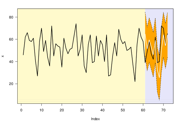
bitmap(file='test1.png')
opar <- par(mar=c(4,4,2,2),las=1)
ylim <- c( min(x[first:nx],lb), max(x[first:nx],ub))
plot(x,ylim=ylim,type='n',xlim=c(first,lx))
usr <- par('usr')
rect(usr[1],usr[3],nx+1,usr[4],border=NA,col='lemonchiffon')
rect(nx1,usr[3],usr[2],usr[4],border=NA,col='lavender')
abline(h= (-3:3)*2 , col ='gray', lty =3)
polygon( c(nx1:lx,lx:nx1), c(lb,rev(ub)), col = 'orange', lty=2,border=NA)
lines(nx1:lx, lb , lty=2)
lines(nx1:lx, ub , lty=2)
lines(x, lwd=2)
lines(nx1:lx, forecast$pred , lwd=2 , col ='white')
box()
par(opar)
dev.off()
prob.dec <- array(NA, dim=fx)
prob.sdec <- array(NA, dim=fx)
prob.ldec <- array(NA, dim=fx)
prob.pval <- array(NA, dim=fx)
perf.pe <- array(0, dim=fx)
perf.mape <- array(0, dim=fx)
perf.mape1 <- array(0, dim=fx)
perf.se <- array(0, dim=fx)
perf.mse <- array(0, dim=fx)
perf.mse1 <- array(0, dim=fx)
perf.rmse <- array(0, dim=fx)
for (i in 1:fx) {
locSD <- (ub[i] - forecast$pred[i]) / 1.96
perf.pe[i] = (x[nx+i] - forecast$pred[i]) / forecast$pred[i]
perf.se[i] = (x[nx+i] - forecast$pred[i])^2
prob.dec[i] = pnorm((x[nx+i-1] - forecast$pred[i]) / locSD)
prob.sdec[i] = pnorm((x[nx+i-par5] - forecast$pred[i]) / locSD)
prob.ldec[i] = pnorm((x[nx] - forecast$pred[i]) / locSD)
prob.pval[i] = pnorm(abs(x[nx+i] - forecast$pred[i]) / locSD)
}
perf.mape[1] = abs(perf.pe[1])
perf.mse[1] = abs(perf.se[1])
for (i in 2:fx) {
perf.mape[i] = perf.mape[i-1] + abs(perf.pe[i])
perf.mape1[i] = perf.mape[i] / i
perf.mse[i] = perf.mse[i-1] + perf.se[i]
perf.mse1[i] = perf.mse[i] / i
}
perf.rmse = sqrt(perf.mse1)
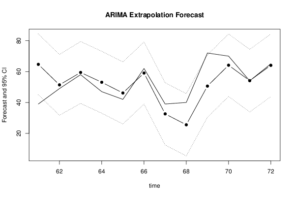
bitmap(file='test2.png')
plot(forecast$pred, pch=19, type='b',main='ARIMA Extrapolation Forecast', ylab='Forecast and 95% CI', xlab='time',ylim=c(min(lb),max(ub)))
dum <- forecast$pred
dum[1:par1] <- x[(nx+1):lx]
lines(dum, lty=1)
lines(ub,lty=3)
lines(lb,lty=3)
dev.off()
load(file='createtable')
a<-table.start()
a<-table.row.start(a)
a<-table.element(a,'Univariate ARIMA Extrapolation Forecast',9,TRUE)
a<-table.row.end(a)
a<-table.row.start(a)
a<-table.element(a,'time',1,header=TRUE)
a<-table.element(a,'Y[t]',1,header=TRUE)
a<-table.element(a,'F[t]',1,header=TRUE)
a<-table.element(a,'95% LB',1,header=TRUE)
a<-table.element(a,'95% UB',1,header=TRUE)
a<-table.element(a,'p-value
(H0: Y[t] = F[t])',1,header=TRUE)
a<-table.element(a,'P(F[t]>Y[t-1])',1,header=TRUE)
a<-table.element(a,'P(F[t]>Y[t-s])',1,header=TRUE)
mylab <- paste('P(F[t]>Y[',nx,sep='')
mylab <- paste(mylab,'])',sep='')
a<-table.element(a,mylab,1,header=TRUE)
a<-table.row.end(a)
for (i in (nx-par5):nx) {
a<-table.row.start(a)
a<-table.element(a,i,header=TRUE)
a<-table.element(a,x[i])
a<-table.element(a,'-')
a<-table.row.end(a)
}
for (i in 1:fx) {
a<-table.row.start(a)
a<-table.element(a,nx+i,header=TRUE)
a<-table.element(a,round(x[nx+i],4))
a<-table.element(a,round(forecast$pred[i],4))
a<-table.element(a,round(lb[i],4))
a<-table.element(a,round(ub[i],4))
a<-table.element(a,round((1-prob.pval[i]),4))
a<-table.element(a,round((1-prob.dec[i]),4))
a<-table.element(a,round((1-prob.sdec[i]),4))
a<-table.element(a,round((1-prob.ldec[i]),4))
a<-table.row.end(a)
}
a<-table.end(a)
table.save(a,file='mytable.tab')
a<-table.start()
a<-table.row.start(a)
a<-table.element(a,'Univariate ARIMA Extrapolation Forecast Performance',7,TRUE)
a<-table.row.end(a)
a<-table.row.start(a)
a<-table.element(a,'time',1,header=TRUE)
a<-table.element(a,'% S.E.',1,header=TRUE)
a<-table.element(a,'PE',1,header=TRUE)
a<-table.element(a,'MAPE',1,header=TRUE)
a<-table.element(a,'Sq.E',1,header=TRUE)
a<-table.element(a,'MSE',1,header=TRUE)
a<-table.element(a,'RMSE',1,header=TRUE)
a<-table.row.end(a)
for (i in 1:fx) {
a<-table.row.start(a)
a<-table.element(a,nx+i,header=TRUE)
a<-table.element(a,round(perc.se[i],4))
a<-table.element(a,round(perf.pe[i],4))
a<-table.element(a,round(perf.mape1[i],4))
a<-table.element(a,round(perf.se[i],4))
a<-table.element(a,round(perf.mse1[i],4))
a<-table.element(a,round(perf.rmse[i],4))
a<-table.row.end(a)
}
a<-table.end(a)
table.save(a,file='mytable1.tab')